Computational Biology Mazen Abdelsttar Seif Eldein Sameh (STEM high school for boys_6th of October)
Astrophysics Reem Zidan | Ahmed Kadry
Artificial Intelligence Kareem Adel Abdelhamid Mohamed | Yahia Mohamed Soliman Hassan Abdelhamid Ahmed Abdelhamid, STEM High school for boys - 6th of October
Engineering Ahmed Hosny | Abylay Iskakov Ziad Ahmed
International Relations and Political Science Akhmetzhan Nurbike | Sapabekova Medina
Engineering Adam Mohamed | Kareem Walid Ahmed S. Ahmed (STEM High School for Boys - 6th of October & Miami University Sophomore)
Politics Ansar Zeinulla
Computational Astrophysics Jana Aboelmagd | Hannah Ragaie
Mathematics Mazen Hisham | Mariam Manaa Hazem Abdel-Mughni (STEM High School for Boys - 6th of October)
Astronomy and Astrophysics Ammar Emad | Abdelhakim Mohamed-Fahmy | Omar Hassan Mustafa Mohammed (STEM High School for Boys – 6th of October)
Psychology Maria Fernanda Souza | Beatriz Mel Carmo, Brazil Salma Elgendy (Maadi STEM School for Girls, Egypt)
Computer Science Abdelrahman Abdelwahab Ahmed Osama (WE for applied technology)
Dear readers,
We are thrilled to present the remarkable works showcased in this issue, a testament to the dedicated efforts of our researchers over the past year. This edition features outstanding projects from our revamped research program as
well as top-rated submissions received through our journal website.
This season, we implemented significant changes to our research program, extending its duration to eight weeks. During this period, junior researchers underwent a thorough and enriching experience, beginning with an intensive
training course that equipped them with essential skills in scientific research, idea generation, and paper writing. Participants engaged in collaborative group projects with peers sharing similar interests, successfully producing
articles within this extended timeframe.
One of the key enhancements this season was the introduction of individual mentoring sessions. Each junior researcher attended these sessions with senior researchers to monitor their progress and apply the knowledge gained
throughout the program. This personalized guidance, coupled with the continuation of group mentoring sessions, provided robust support as the teams developed their inaugural review papers.
Following the completion of their projects, each group presented their findings in concise 10-minute sessions to a distinguished panel of judges. The depth of ideas and the quality of the projects were truly commendable.
Participants received constructive feedback that highlighted their performance in key areas such as defining a research question, methodology, and presentation skills, demonstrating their dedication to academic excellence.
Our editorial team also diligently reviewed numerous papers submitted to the Youth Science Journal website for publication. After a rigorous revision process, we reached out to the authors of papers that showcased academic novelty
and significant contributions to their respective fields. We are excited to feature articles from various STEM and Humanities disciplines, including interdisciplinary ones, and we look forward to the continued review of submitted
articles.
This issue proudly presents the exceptional group projects created during the extended training program and the selected submissions from our website. We express our deepest gratitude to our senior researchers for their invaluable
mentoring and extend heartfelt thanks to all contributors who made this publication possible.
Best Regards,
Youth Science Journal Community
A Comparative Study of the Perceived Stress Levels and Sources of Stress among STEM and Conventional Students in Egypt
Salma Alkosha (Maadi STEM High school for girls)
Zeinab Yasser | Omar Aboolo (STEM High School for Boys - 6th of October)
Abstract
Egypt's educational system, comprising public and private institutions across all levels, faces multiple issues affecting its quality, equity, and relevance. A recent study by Egypt's Ministry of Health identified that 29.8% of
high school students experience mental health problems like anxiety, speech defects, depression, stress and tension, emphasizing the significance of addressing such concerns. Therefore, we aimed to conduct a random sample study of
130 students from the STEM and conventional educational systems in Egypt to compare their perceived stress levels. An online Arabic questionnaire was shared with the targeted population over a period of two weeks. The
questionnaire included inquiries about academic and demographic information as well as the Perceived Stress Scale (PSS-10). Respondents were asked about their personal information, academic performance, extracurricular activities,
average studying hours, and perceived stress levels. The PSS-10 assessed stress levels based on questions covering coping, control, unpredictability, and overload. Statistical analysis was conducted using the Statistical Package
for the Social Sciences (SPSS) version 25. Major findings revealed that STEM students suffer from higher stress levels than conventional students, mainly due to fewer hours of sleep. Additionally, significant differences were
found in stress levels between male and female students across the sample. These findings underscore the need to address academic pressures and establish appropriate mental health screening in STEM schools to mitigate negative
emotional effects. They are crucial in developing effective strategies for minimizing student stress levels, and educational institutions should utilize this data to assess their curriculum and make any necessary changes.
As we navigate through the academic jungle, it's no secret that we may encounter academic-related stress, which is an aspect of most Egyptian students' life. A new study published by Egypt's Ministry of Health reveals that 29.8%
of high-school students suffer from anxiety, tension, speech defects, or depression disorders. Deadlines, parental and societal pressure, desire for perfection, and poor time management are among the most common causes of stress
among high school students.
Egypt's educational system is one of the biggest in Africa and the Middle East, comprising both public and private institutions at primary, preparatory, secondary, and tertiary levels. Despite governmental efforts to improve
education, however, the system continues to be riddled with several problems that negatively affect overall mental health among students. Egypt's high school system offers diverse programs geared toward career fields, including
general, vocational, and technical education.
Despite the significant efforts in the field of educational psychology, no previous studies- to the best of our knowledge- have addressed the difference between stress levels among STEM schools students in Egypt and conventional
schools, taking into account the learning system, the social interactions, extracurriculars, personal habits, and extra projects and tasks.
Therfore, this study aims to compare the prevalence of perceived stress among two major educational systems in Egypt, STEM high schools and conventional high schools, as they differ in academic advancement levels, curriculum,
teaching methods, extracurriculars, skills, and knowledge they aim to impart. As well as determining and analyzing possible demographic and academic factors related to stress levels among both populations.
The methodology involved conducting an online Arabic survey asking for necessary demographic and academic information as well as the ten questions of the Perceived stress scale. Data were collected from 130 respondents, including
males and females, STEM and non-STEM students, various academic levels, and educational grades. Data were analyzed to examine the difference in stress levels between both populations and the significance of association between
stress levels and other variables.
Ensuring that the study is designed ethically and fairly to benefit students and educational institutions in Egypt, we will ensure that the findings and results of the study can be practically implemented in educational
administrations.
Hypothese
Null Hypothesis (1): There will be no statistically significant difference between STEM educational system's students and the conventional educational system's students regarding perceived stress levels.Null Hypothesis (2): There will be no statistically significant difference between males and females regarding perceived stress levels.Null Hypothesis (3): There will be no statistically significant difference between different educational grades (Grades 10 & 11 & 12) in terms of perceived stress levels.
II. Literature Review
Intensive research and experiments have been conducted to find the relation between academic performance and stress (including psychological, physical, social, and academic stress). Previous research has indicated a significant
negative impact of stress on academic performance, which was roughly equal between males and females, ensuring that teachers play a vital role in reducing stress among their students
[1]. Indirect stress may develop due to task load requirements
[2]
, and stressed students tend to be slower and more considerate in their actions
[3]
. Stressors are widely spread among secondary school students in boarding schools; specifically, about 44.9% of pupils experience academic-related stressors
[4].
To reduce levels of stress, experiments have been conducted on the effect of extracurriculars on reducing the amount of stress among high school students, and the results showed that students who participate in extracurricular
activities show fewer levels of stress and worry
[5]. Other studies showed that participation in extracurricular activities moderates the relation between academic related stress and coping and positively influences well- being
[6]. Further approaches to reduce stress levels among students include developing social interactions with family, friends, and society. A preceding study has indicated that levels of stress among high school students were
significantly predicted by family support, whilst levels of depression were significantly predicted by friends' support
[7]. Another study comparing between conventional and boarding schools concerning their social activities has indicated that conventional school students showed higher levels of peer-group integration than students from boarding
schools, on the other hand, boarding school students showed higher success in gaining autonomy from parents and forming romantic relationships
[8]
.
III. Methodology
1. Participants
This research employs a mixed online survey that lasted for two sequential weeks starting from the 11th of August, 2023. It was used to obtain data from a random sample of students from both the conventional educational
system and STEM educational system in Egypt. 130 anonymous responses were collected from various high schools and localities in Egypt.
2. Measurements2.1. Demographics: Respondents were asked to fill in their personal information, including birth date, gender, and average sleeping hours. 2.2. Academic Information: Respondents were asked about their academic performance, extracurricular activities during school months, average studying hours, educational system, educational level, as well as their
academic grades.
2.3. Perceived Stress Scale ( PSS-10): The perceived stress scale (PSS) is a structured questionnaire used for assessing the level of stress that a population or a sample of it faces during a specific period. The
test includes ten questions that cover topics such as coping, control, unpredictability, and overload. Questions such as " In the last month, How often have you felt that you were unable to control the important things in your
life? " were asked, and the respondent was required to give an answer on a scale from 0 (Never) to 4 (Very Often). The final score will be the sum of the scores of each question by reversing the scores of questions 4, 5, 7, and 8.
Where in these four questions, a score of 4 is actually 0, 3 is 1, 2 is 2, 1 is 3, and 0 is 4. A final score of 0-13 indicates low stress levels, 14-26 indicates moderate stress levels, and 27-40 indicates that the respondent
suffers from severe stress.
3. Procedures
In order for the data to be collected effectively, a structured online validated Arabic questionnaire of multiple choice questions was done using Google Forms. It was accessible to the targeted populations and sent to them via
social media and mail platforms, for instance, WhatsApp and Microsoft Outlook. Daily reminders for filling out the form were sent as well.
Participants' responses, which included concise/clear answers for the demographic, academic information, and PSS-10 sections, were recorded. Two weeks later, data were collected and begun to be analyzed. 4. Data collection and instrumentation
The collected data represented the score of stress of each individual, as well as other necessary information for testing the hypotheses. All analytic processes were done using the Statistical Package for the Social Sciences
(SPSS) version 25 tool. Descriptive statistics tests were done to determine similarities and differences among both populations.
Table [1]
shows statistical methods used to compare between both populations (STEM & non- STEM).
Table [2] >
shows statistical methods used to determine the relation between different demographic/ academic variables and stress scores.
Table [1] : Statistical tests used to compare between STEM & non- STEM.
Variable
Statistical Test
Variable
Statistical Test
Age
Independent sample t-test
Stress Score
Independent sample t-test
Educational Level
Chi-Square test
Sleeping Hours
Chi-Square test
Gender
Chi-Square Test
Sudying hours
Chi-Square test
Number of extracurriculars
Mann-Whitney
Categories of extracurriculars
Mann-Whitney test
Academic performance
Chi-Square test
Table [2] : Statistical tests used to determine the relation between different demographic/ academic variables and stress scores.
Relations
Dependent Variable
Independent Variable
Statistical Test
Gender * Stress Score
Stress Score
Gender
(Males & Females)
Independent sample t-test
Educational level * Stress score
Stress Score
Educational Level
(Grades 10 & 11 & 12)
Oen Way ANOVA
Sleeping hours * Stress score
Stress Score
Sleeping hours
(< 4) & (4-8) & (> 8)
Oen Way ANOVA
Post Hoc tests — Tamhane test
Studyinh hours * Stress score
Stress Score
Sleeping hours
(< 6) & (6-12) & (> 12)
Oen Way ANOVA
Categories of extracurriculars * Stress score
Stress Score
Number of difference categories of extracurriculars (1-7)
Spearman's correlation coefficient test
Number of extracurriculars * Stress score
Stress Score
Number of extracurriculars
Spearman's correlation coefficient test
Educational system * Stress score
Stress Score
Educational system
(STEM & non-STEM)
Independent sample t-test
IV. Results
1. Demographic Analysis
A total of 130 responses were collected from conducting the online survey. Respondents included 83 females (64%) and 47 males (36%). STEM students represented 61% (79 students), while conventional (non- STEM) students represented
39% of respondents (51 students). The academic performance of the majority of respondents (92students) ranged between 80-89%, 34 students ranged between 90-100%, while only 4 students were between 70-79%. Most of the respondents
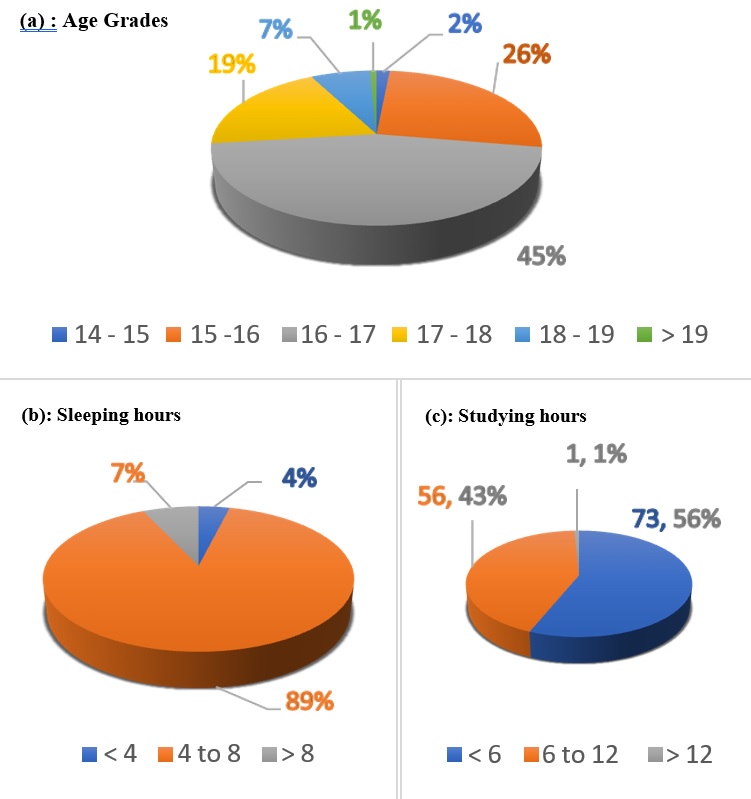
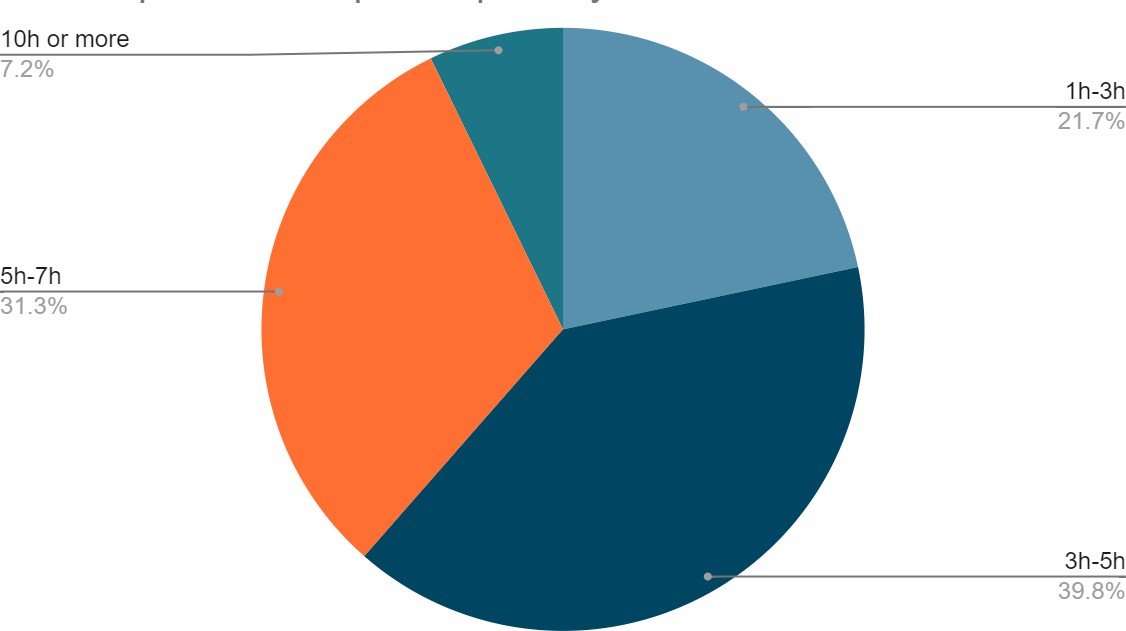
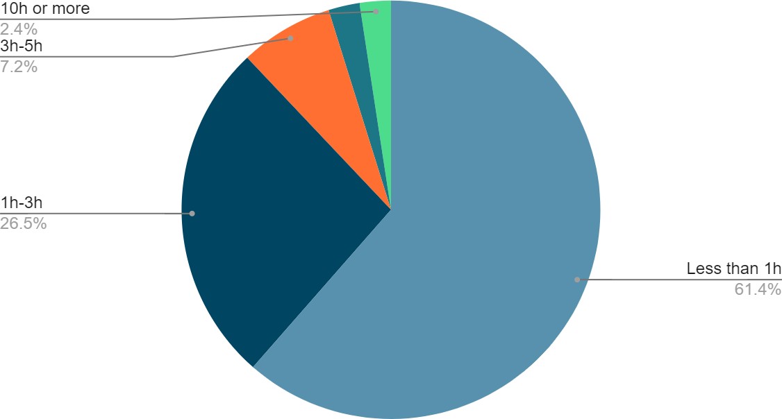
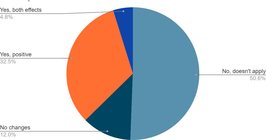
(92 students, 71%) aged between 15- and 17-years Fig. (1). 69% of respondents (90 students) were in grade 11, 20% (26 students) were in grade 12, while 11% (14 students) were in the 10^th^ grade. Average sleeping hours
for most of the students (116 students, 89%) ranged between 4-8 hours/day, while average studying hours for the majority of students (73 students, 56%) was less than 6 hours/ day Fig. (1).Fig. (1): Demographic Information
(a): The distribution of recorded age grades of the sample. 2 students were aged between 14 -- 15 years, 34 students were between 15 -- 16, 59 students were between 16 -- 17, 25 were aged between 17 -- 18, 9
students were between 18 -- 19, and only one student was above 19 years. (b): Shows the average sleeping hours among students. 5 students used to sleep less than 4 hours/day during school months, 116 students
used to sleep 4 to 8 hours/day, while 9 students used to sleep more than 8 hours/day. (c): This pie chart illustrates the average studying hours of the two populations. Only one student used to study more than
12 hours/day, 56 students used to study 6 to 12 hours/day, while 73 students used to study less than 6 hours/day.
Table [3]
below indicates that there was no statistically significant difference between age, gender, educational grade, and studying hours between both populations. However, there was a statistically significant difference between academic
performance, sleeping hours, number of extracurricular activities, and the variety of their categories.
Table[3] : Demographic information comparison between both educational systems.
STEM
Non-STEM
P value *
Age (mean ± SD)
16 ± 0.925
16 ± 0.947
0.979
Gender (M/F)
11/54/14
3/36/12
0.300
Academic performance
A (90-100%)
B (80-89%)
C (70-79%)
10 69 0
24 23 4
< 0.001
Study hours
< 6 hours
6-12 hours
> 12 hours
38 40 1
35 16 0
0.060
Sleep hours
< 4 hours
4-8 hours
> 8 hours
3 75 1
2 41 8
0.007
Activity Categories
None
1
2
3
4
5
6
7
1
8 5 14 18 13 10 10
6
18 11 7 4 2 1 2
< 0.001
Number of activities (mean rank)
76.65
46.59
< 0.001
*The mean difference is significant at the 0.05 level.
2. Perceived stress scale Responses Table [4]
below shows the responses of 130 students to the perceived stress scale questionnaire, the questions from 1 -- 10 correspond to the validated PSS -10 copy.
Table [4]: PSS -- 10 responses
Question Number (Count, Percent)
0 (Never)
1 (Almost Never)
2 (Sometimes)
3 (Fairly Often)
4 (Very Often)
Question 1
5
(3.8%)
11
(8.5%)
45
(34.6%)
46
(35.4%)
23
(17.7%)
Question 2
5
(3.8%)
14
(10.8%)
29
(22.3%)
53
(40.8%)
29
(22.3%)
Question 3
2
(1.5%)
6
(4.6%)
20
(15.4%)
45
(34.6%)
57
(43.8)
Question 4
9
(6.9%)
24
(18.5%)
49
(27.7%)
28
(21.5%)
20
(15.4%)
Question 5
14
(10.8%)
51
(39.2%)
45
(34.6%)
17
(13.1%)
3
(2.3%)
Question 6
4
(3.1%)
14
(10.8%)
32
(24.6%)
57
(43.8%)
23
(17.7%)
Question 7
17
(13.1%)
32
(24.6%)
55
(42.3%)
19
(14.6%)
7
(5.4%)
Question 8
19
(14.6%)
51
(39.2%)
37
(28.5%)
16
(12.3%)
7
(5.4%)
Question 9
4
(3.1%)
12
(9.2%)
19
(14.6%)
50
(46.2%)
35
(26.9%)
Question 10
5
(3.8%)
11
(8.5%)
30
(23.1%)
36
(27.7%)
48
(36.9%)
3. Relation between demographic variables and stress levels.
Table (5): Significance of association of respondents' demographic/academic variables with stress score
Stress Score Mean
Standard Deviation
P value
Significance of Association with Stress Scores
Educational System
STEM
Non-STEM
26.4935
24.3000
5.69770
6.51920
.047
Statistically significant
Gender
Females
Males
27.0370
23.1522
5.69527
6.06984
< .001
Statistically significant
Educational Grade
Grade 10
Grade 11
Grade 12
23.6429
25.5455
27.0400
5.59680
6.34254
5.33448
.244
Statistically significant
Studying Hours
< 6hrs.
6 — 12 hrs.
> 12 hrs.
5.3857
25.9286
6.42976
5.77410
.884
Statistically significant
Sleeping Hours
< 4hrs.
4 — 8 hrs.
> 8 hrs.
30.0000
25.7965
21.1111
3.67423
6.05209
5.66667
.021
Statistically significant
Mean Square
df
Grade (Among STEM population)
26.697
2
.445
Statistically significant
Grade (Among non- STEM population)
78.644
2
.158
Statistically significant
a. stress score is constant when study hours = 12 hours. It has been omitted.
There was a statistically significant negative relation between sleeping hours and stress levels.
Table [5]. Post Hoc -- Tamhane test indicated that the difference is mainly between individuals who sleep less than 4 hours and those who sleep more than 8 hours.
Table [6].
Table [6] Post Hoc tests - Multiple Comparisons
Sleep Hours
Sleep Hours
Mean Difference
Sig.
Tamhane
< 4 hours
4-8 hours
4.20354
.170
> 8 hours
8.88889*
.013
4-8 hours
< 4 hours
-4.20354
.170
> 8 hours
4.68535
.116
> 8 hours
< 4 hours
-8.88889*
.013
4-8 hours
-4.68535
.116
Table [7] : Correlation between the number of extracurriculars/ their categories and stress scores
Spearman's rho'
P -value
Significance of Association with Stress Scores
Categories of extracurricular activities * Stress Score
.038
.674
Statistically insignificant
Number of extracurriculars * Stress scores
.036
.686
Statistically insignificant
4. Linear Regression Analysis
Linear regression test was performed using those variables significantly associated with stress in univariable analysis as independent variables (i.e.:gender, educational system and sleeping hours), while stress scores were used
as the dependent variable. The regression revealed that gender and sleeping hours were significant predictors of stress (p values <0.001 and 0.026, respectively), while educational system showed only marginal significance as a
predictor (p value = 0.086).
V. Discussion
This current study aims to compare stress levels between STEM and Conventional students in Egypt and identify the significance of association of certain demographic and academic factors with stress levels among both populations.
Null Hypothesis (1): There will be no statistically significant difference between STEM students and conventional students in terms of perceived stress levels.
According to the findings of this study represented in
table [5], this hypothesis was rejected as there was a statistically significant difference between means of stress levels between both populations (p = .047). This is closely related to the nature of STEM schools in
Egypt as being boarding schools for excellent students and associated with higher levels of competition and extracurriculars than conventional schools -
table [3] .
Previous studies have addressed the effect of being educated in a boarding school on stress levels and social interactions. Children sent to boarding schools tend to suffer from sudden and often irrevocable traumas, as well as
bullying and sexual abuse
[9]. One study analyzing the societal interactions of both boarding and day schools' students has shown that boarding schools' students reported higher success in gaining autonomy from parental environments as well as higher ability
in forming romantic relationships than day schools' students. On the other hand, adolescents from day schools scored higher ability in peer- interactions and greater parental support
[9]. Peer relationship has a great ability to reduce academic stress (t = - 38.62, p < 0.001) among students
[10]. The same study revealed the significance of parental support in handling stress among children. The study's findings showed that the parent-child relationship can negatively predict academic pressure (t = - 56.29, p < 0.001).
The lack of the previous two factors (parental and peer relationships) may be among the causes of the elevated stress scores among STEM students than conventional students.
STEM students in Egypt tend to participate in a variety of extracurriculars with higher levels than their non-STEM counterparts
table [3]. The reason behind this is the intensive competition present between STEM students in terms of academic achievement, seeking for scholarships, and enhancing their experience and knowledge. Too many assignments,
close deadlines, and dropping entertainment activities because of schoolwork were reported to be significant sources of stress among 61% of students
[11], which are sources believed to be associated with extreme participation in extracurriculars. On the other hand, previous studies have indicated the influence of participating in extracurriculars on reducing academic stress
levels. One study has indicated that there is a slightly negative correlation between extracurriculars and stress / suicidal ideation (r = −0.083, p < 0.001), (r = −0.039, p < 0.01) respectively
[12]. Another study has shown that participating in extracurricular activities has a significant positive influence on academic outcomes, as well as moderating the relationship between academic stress and coping
[6]. Despite these studies, our findings have not shown a significant correlation between number of extracurriculars or the variety of their categories and the reduction of stress levels (P = .686) (P = .674), respectively.
Table [7] .
STEM students, when participating in extracurriculars, tend to reduce their sleeping hours instead of studying hours to cope effectively with the responsibilities that are required by extracurriculars and to balance between
academic excellence and other activities. Our findings
table [3] , have indicated that there is a significant difference in sleeping hours between STEM and non- STEM students (P = 0.007), while there was no statistically significant difference but a tendency between studying
hours among both populations (P = 0.060). On the other hand, results in
table [5]
have indicated a significant association between sleeping hours and elevated stress levels, indicating that decreasing sleeping hours significantly increases stress levels among students ( P =.021), while no statistically
significant association was present between studying hours and elevated stress levels ( P = .884), which is indicated by prior studies that revealed that there was a weak correlation between stress and study hours (r = 0.062)
[13]
. Post Hoc -- Tamhane test
table [6]
shows that a significant difference in stress levels is present specifically between students who sleep less than 4 hours per day and those who sleep more than 8 hours (P = .013). At the same time, no statistically significant
difference was present between those who sleep less than 4 hours or more than 8 hours and those who sleep between 4 to 8 hours per day. The significant association between sleeping hours and stress levels was indicated by several
previous studies. Prior findings have shown that 80.2% of high school students in Lukasa were stressed due to a lack of quality and quantity of sleep
[11]. Many students tend to be exhausted, and they get significantly less than the recommended 9 hours of sleep, 70% of them reported that they were often or always stressed by workload
[14]
. Poor quality sleep is proven to be significantly associated with elevated mental stress levels as well (p < 0.001)
[15].
Null Hypothesis (2): There will be no statistically significant difference between males and females in terms of perceived stress levels.
This hypothesis was rejected by the outcome results represented in
table [5],
which indicates there was a statistically significant difference (<0.001) between males and females in terms of perceived stress levels. This finding is consistent with the findings of a preceding study which revealed that
women were more likely than men in experiencing higher levels of stress
[16]
. For more specification, a previous study has indicated that women score higher levels of stress on the PSS -10 compared to their male counterparts
[17]
. This study has indicated that self- distraction, emotional support, venting, and instrumental support were common ways among students and especially females to cope with stress states and perceive temporal relief from stressors.
One study has shown that Egyptian female dental students score higher levels of stress than males due to personal and clinical factors, workload, and performance pressure
[18]
. Another study done on high school students in Lusaka revealed that upon the conduction of the questionnaire, 62% of males reported being stressed because of domestic responsibilities compared to 81.5% of females
[11]. On the other hand, other findings indicated that females were better than males in handling academic stress
[19]
. Another study has indicated that higher secondary male students are subjected to higher academic stress levels than their female counterparts
[20]
. Furthermore, a neutral finding has indicated that there was no statistically significant difference between males and females on the perceived stress scale
[21]
. Past studies have suggested several reasons behind females being more subjected to stress. Daily stress associated with routine role functioning, gender caring role-related stress, gender violence, sexist discrimination, being
more emotionally involved than males in social networks, and being affected by others' stress, are among the significant sources of stress to females
[22]
.
Null Hypothesis (3): There will be no statistically significant difference between different educational grades (Grades 10 & 11 & 12) in terms of perceived stress levels.
According to the results shown in
table [5],
there was no statistically significant difference in perceived stress levels among the three populations (grades 10 & 11 & 12) (P = .244). Although by comparing means of stress levels among three populations, it can be inferred
that means of stress levels have increased by the advancement in educational level, (Grade 10: Grade 11: Grade 12) = (23.6429: 25.5455: 27.0400). Therefore, this hypothesis was approved by the results. These findings contradict
previous studies that aimed to compare different educational grades in terms of stress levels among high school students as well as university students. One study has indicated that 28% of grade 11 students experience high or
extreme stress compared to 26% of grade 12 students, indicating that significant stressors included lack of time for revision, queries from society, and parental expectations
[23]
. Variety in these factors may be the reason behind the difference in the findings. Other findings have shown that junior university students experienced higher perceived stress levels than senior students (M=18.49, SD=5.46) & and
(M=15.58, SD= 5.36), respectively
[21]
. On the other hand, a contradictory study to the previous findings revealed that mid-senior Egyptian dental students showed some higher stress levels than junior students
[18]
.
Upon performing the linear regression test, findings revealed that sleeping hours and gender are significant predictors of stress, while educational system was found to be not a major cause and a significant predictor of stress
among high school students.
Poor sleep is proven by previous findings to be a significant predictor and closely related to stress. A preceding study done on King Abdulaziz University's students have shown that upon the preforming an electronic
self-administered questionnaire, results indicated that 65% of students experienced stress, while 76.4% of them suffered from poor sleep quality. Findings revealed that the increase in stress levels is a significant predictor of
stress (Cramer's V = 0.371, P < 0.001)
[24]
. Another study done on medical students have shown that 76% of students were suffering from poor sleep quality, and 53% of them were suffering from elevated stress levels. Logistic regression test has revealed that students who
do not experience stress are less likely to have poor quality of sleeping states
[25]
. Sleep deprivation or Insomnia triggers the body to release Cortisol hormone during day hours, and potentially to maintain an alert state of the body. Sleep and stress responses are greatly associated in the physiology of human
body, as both share the the hypothalamic- pituitary-axis (HPA). A disruption in the function of HPA leading its axis to be acute can disrupt sleeping cycles. Upon experiencing prolonged or chronic stress, hypothalamus and
pituitary glands send messages to the adrenal gland to secrete more cortisol, leading to an overly active HPA axis.
Major findings of this study have revealed the significant difference in stress levels between STEM and non-STEM students and suggested that a possible reason is that over-participating in extracurricular activities by STEM
students has reduced the quality and quantity of sleeping hours, which is significantly associated with elevated stress levels. On the other hand, participation in extracurriculars hasn't affected study hours between both
populations, which was found to be not significantly associated with elevated stress levels. Females have shown higher stress scores than their male counterparts on the PSS. And it is found that advancement in educational level
was not significantly associated with elevated or reduced stress levels in general. The same results were found when splitting the sample upon the educational system and examining the relation between educational levels and stress
scores in each population independently
table [4].
Further studies that are concerned with similar topics and aspire to build upon this study may be concerned with determining stress differences between the genders more thoroughly, within STEM students or non-STEM students
independently, to examine if there is a difference in coping abilities between males and females in both educational systems.
As the data reveal, there is no association between stress levels and extracurricular activities; nevertheless, further studies may be employed to determine if there is a specific sort of extracurricular activity that relieves
stress, such as physical, literary, or social activities.
The study's findings may be shared with educational institutions, including teachers and administrators, to investigate possible methods to minimize student stress levels as the outcomes of the study could be used by educational
departments to assess their curriculum and make the necessary adjustments.
The study findings revealed that STEM students suffer from elevated levels of perceived stress compared to their non-STEM counterparts, psychological guidance is required, and mental health instructors should be present in the
educational environment to asses students overcome psychological problems when faced.
During the research process, there were certain situations in which we faced some limitations. For instance, recall bias, is a serious risk that can potentially influence the validity of survey data. It usually occurs because of
individuals' failure to recall or recount their experiences, which can lead to errors in their responses. This risk could be considerable since the research variables' most recent encounter was three months ago. An approach to
reduce recall bias was to employ multiple-choice questions with all possible responses that could aid respondents in remembering their answers. Another important limitation was represented in the limited number of responses, a
total of 130 responses may be inefficient enough to come up with strong and reliable data despite the significant effort made to widen the spread of the questionnaire and the daily reminders sent to respondents. However, there was
a remarkable lack of responses that may decrease the findings' validity. In spite of lack of responses, the findings were consistent to a great extent with previous findings in the same feild. Future reseach can be conducted
employing a greater number of respondents to ensure the validity of the data. Furthermore, the original copy of the PSS-10 requires responses to situations that have occurred a month before. However, we have utilized the PSS-10
questionnaire in structuring an online survey that was concerned with situations that happened during a 3- month period before. A limitation that may influence negatively the accuracy of responses. However, we considered the
employment of MCQs to reduce the recall bias.
Moreover, the research was concerned with Egyptian students and educational systems. Taking into account socioeconomics and cultural themes, it was hard to identify earlier literature studies on related topics that represent
reliable findings closely related to the study topic. Nevertheless, similar socioeconomic and cultural conditions were maintained during researching in the literature.
Finally, the short time frame for collecting data, conducting the analysis, and discussing results and recommendations was a great challenge during the research process.
IV. Conclusion
This study was the first of its kind aimig to assess the variation in the prevalence of perceived stress between two types of educational systems in Egypt: STEM and conventional secondary systems. Taking into consideration social,
academic and extracurricular factors, and utilizing a significant number of statistical tests for data analysis. The sample (130 high school students) was chosen randomly, and respondents were asked to fill in an online Arabic
survey to identify specific demographic information and determine stress score through the perceived stress scale -- 10. The analytic tests done on the results revealed that STEM students are subjected to higher levels of
perceived stress than conventional students. Lack of strong parental relationship, excess workload, and intensive competition contribute to this significant difference in stress levels. However, the most important factor was the
lack of quality and the reduced quantity of sleep hours, which may be a result of over participating in extracurriculars. Additionally, we found that there was a significant difference between the two genders in terms of stress
levels. Upon analyzing the influence of these factors on the overall mental health of students, addressing them and establishing appropriate mental health screening in STEM schools is an essential step that may aid in developing
the creativity, innovation, and enthusiasm of students and reducing negative emotional and mental problems that may affect academic or social performance among students.
V. References
[1]
A genetic approach for tackling sickle cell disease
Mohamed Mohamed | Mo'men Emam
(STEM High School for boys-6th of October.)
Abstract
SCD is a serious inherited hemoglobinopathy that was responsible for the mortality of 376000 patients in 2021. The number of infants born with this genetic disorder was raised by 13.7% within the time interval from 2000 to 2021.
Its fetal complications and painful VOC episodes are associated with a reduced quality of life and hospitalization and healthcare burden. Most SCD therapies are symptom-managing focused rather than curing the disease itself. This
study mainly focused on the most life-threatening complications including cardiovascular complications and acute splenic sequestration, medications managing or curing them including hydroxyurea (HU) and gene therapy. HU was found
to be effective in reducing cell sickling and was associated with improvements in organ functions represented in decreased acute chest syndromes and crises requiring blood transfusion. Its drawbacks were obvious in reduced sperm
count and restricting erythroid cells' growth. Curing SCD gives lentiviral Gene therapy an advantage compared to HU. However, more research should be done on developing gene therapy to find out the reason and solution of
malignancies reported in some cases.
I. Introduction
The disease of sickle cell anemia (SCD) was common in Africa for about 5000 years. A story of researching, discovering complications, and finding out medications, was written by great scientists, like chemist Dr. Linus Carl
Pauling, Dr. Ingram, and others, to make an evolution from calling patients "ogbanjes" in Africa to the use of gene therapy techniques to treat it
[1]. The disease is related to hemoglobin mutations that cause many disorders including sickle cell anemia. This disease starts with a single mutation in hemoglobin creating sickle cell hemoglobin (HbS). As a result, the shape of
blood cells (from the name of the disease, sickle cell anemia) becomes crescent-like by a process of sickling the blood cells by interactions among erythrocytes, leukocytes, thrombocytes, and vascular endothelium. That leads to a
blockage in the bloodstream resulting in dangerous complications and can lead to death. The complications have different levels, and some may not require hospital visits and others require intensive care units (ICU)
[12]. Cardiovascular complications and acute splenic sequestration are some of those that can lead to death in both adults and children. Cardiovascular complications are clearly related to SCD by the fact that SCD can cause blockage
near the heart. These complications can lead to a low supply of oxygen to the body leading to hard pain and high anemia. Because of the body's need for oxygen for its main functions, SCD affects those functions badly. Also, the
spleen has an important role in the human body as it deals with dead blood cells. So, it is easily affected by closing splenic veins, by Vaso-occlusion, resulting in a complication called acute splenic sequestration (ASS). It
leads to low hemoglobin levels, anemia, enlargement in the spleen size, probably splenectomy, and a mortality rate greater than 20 %. Generally, fetal hemoglobin (HbF) is known for its ability to reduce the effect of SCD
[6]. That encouraged the researchers develop a medication called hydroxyurea. This medication can solve many of the cases and people who stick to it are predicted to have a longer life than others who don't stick to it. When the
level of HbF becomes in- between 20% and 33%, SCD has no effect on the patients. However, some patients don't respond to this medication positively and others have no effects at all. Another group of patients respond negatively
and some of the complications deteriorate. So, scientists recommend only the minimum effective level of this therapy to avoid these negative cases
[12]. Another studied medication is lentiviral Gene therapy. It depends on the gene addition method, by lentiviral vectors, to reduce the effects of HbS. Its bad side effects are not popular, making it a recommended treatment for
SCD.
II. Hemoglobins
The human hemoglobin (Hb) is the factor that controls how the human body will be. Characteristics like length, eye color, and others have resulted from its function. There are many types of hemoglobin in humans. Some of them are
healthy and normal and others are abnormal and can cause many disorders
[1]. Mainly, the normal hemoglobins are adult hemoglobin (HbA), fetal hemoglobin (HbF), and HbA2. Typically, they consist of two different parts, which are Heme and Globin. Heme is a combination of an iron atom and porphyrin. The
term porphyrin means a heterocyclic tetrapyrrole ring system. The four rings of porphyrin are connected, cyclically, by methene bridges
[21]
. Globin is made up of 2 alpha chains and 2 beta chains. This is HbA (α2 β2). Other normal hemoglobin types are HbA2 (α2δ2), which has 2 delta chains instead of the beta chains, and HbF (α2γ2), which has 2 gamma chains instead of
the beta chains. The alpha chain consists of 141 amino acids and the origin of the two chains is the alpha gene cluster of chromosome 16, while beta chains are comprised of 146 amino acids and their origin is the beta gen cluster
in chromosome 11
[6]. Adult hemoglobin (HbA) and fetal hemoglobin (HbF) have similar genes since they exist on chromosome 11. However, HbF production decreases in an accelerated manner after birth. In the healthy conditions, adults have 96:98%,
<3.5%, and <1% of HbA, HbA2, and HbF respectively. In addition, HbA2 is just a minor component in the blood cells in humans. So, HbA is specifically the normal one after birth
[21]
.
Sickle cell anemia patients have a high percentage of abnormal hemoglobin called hemoglobin S (HbS). HbS is different from HbA as HbS has a valine in the 6^th^ position in the beta chains instead of amino acid. So, this mutation
causes the "sickle cell disease"
[6]
III. Sickle Cell Anemia
i. Sickle cell anemia history
Sickle cell anemia was common in Africa for about 5000 years but that was not recorded well
[1]. Some scientists believe that the origin of SCD mutation happened about 70—150,000 years ago. It is known that the term "ogbanjes" was used by African people to describe weak babies who were sickle cell anemia patients in the
distant past
[6]. Over the last two centuries, there were observations on humans and animals that led to the full discovery of sickle cell anemia. Firstly, in 1840, at the London Zoological Garden, a scientist called Gulliver noticed strange-
shaped red blood cells in the blood cells of the deer in the garden
[4]. They were crescent or sickle- shaped. At the same time, the white-tailed deer in North America in the forests of Michigan were dying because of Vaso-occlusive problems. In 1905, two French scientists published a report about
"half- moon corpuscles" in the blood of 5% of 243 local Algerians who were anemia patients. The scientists wrongly related these sickle erythrocytes to malaria instead of SCD. Also, in 1904, a patient called Walter Clement Noel
visited the hospital of Chicago Presbyterian since he was suffering from an ulcer on his ankle
[1]. His physicians were James Bryan Herrick and his intern Ernest Eddward Irons
[6]. After checking Noel's blood, Dr. Irons noticed strange blood cells and named them "peculiar, elongated, and sickle-shaped". So, by the end of 1910, Dr. Herrick connected the abnormalities in the red blood cells' shapes to the
sickle cell anemia disease when he reported on "Peculiar Elongated and Sickle-Shaped Red Blood Corpuscles in a Case of Severe Anemia" in the "Archives of Internal Medicine". That was the first time to do so, as a result, 1910 is
described as the discovery year of sickle cell anemia disease
[1]. The first scientist who denominate the disease by "sickle cell anemia" was Verne Raheem Mason in 1922
[6]. In 1927, it was discovered that removing oxygen makes red blood cells of patients, with sickle cell anemia, sickle. In addition, some of the patients' families' blood cells were sickling by removing oxygen although they had no
symptoms. So, those people were called "sickle traits". That was the first discovered cause-effect relationship between the sickling of sickle cells and acidic conditions and low oxygen, by two scientists called Hahn and Gillespie
[10]. In 1949, other two physicians, called Dr. James V. Neel and Col. E. A. Beet, proved that sickle cell anemia is an inherited disease that the patients are homozygous and carry two alleles of sickle cell anemia while sickle cell
traits are heterozygous and carry one allele of sickle cell anemia
[1]. In the same year, the famous chemist Dr. Linus Carl Pauling with his co-worker Dr. Harvey discovered the cause-effect relationship between an abnormality in the chemical structure of hemoglobin molecule and sickle cell anemia
[10]. Sickle cell anemia is the first disease that took the name "molecular disease". This term was coined by Dr. Linus Carl Pauling and Dr. Harvey after their findings. Thanks to this discovery, Dr. Linus Pauling received a Nobel
Prize in 1954
[1]. After two years, the details of the irregularity of hemoglobin in sickle cell patients were discovered clearly by a scientist called Dr. Ingram. In 1956, he found that the 6^th^ position of the amino acid chain has amino acid
valine instead of glutamic. Counting from the amino- terminal, that 6^th^ position was the only strange one on the whole amino acid chain of SCD patients' blood
[6]. That was one of the most important discoveries in sickle cell anemia. In the following years, more details were discovered, and the complications were clearly related to the disease itself. It was found that the mutation of
glutamine-to- valine substitution happens in the beta-globin chain at chromosome 11. To ensure supporting SCD patients and their families Dr. Charles F. Whitten in the 1970s helped the "Sickle Cell Disease Association of America"
(SCDAA) to be founded. Nowadays, 90% and 50% of SCD patients can live to the age of 20 and 50 respectively. The average age of SCD patients is about 58 years for women and 53 for men. This indicates the improvement in curing and
supporting SCD patients. Because in the past, "ogbanjes" were dying at an early age
[1].
ii. Pathophysiology of SCD
The pathophysiology of sickle cell anemia starts with the arising of Sickle cell hemoglobin (HbS). That happens because of the mutation in the hemoglobin (Hb) beta chain, as at the 6^th^ position, it has the amino acid valine,
while the normal one is glutamate. This glutamine-to-valine substitution occurs as a result of an original mutation when the 6^th^ codon in the beta- globin chain has thymine instead of adenine
[25]
. This mutation creates the HbS and enables it to form polymers under deoxy conditions
[13]. In addition, it causes abnormality in molecular stability and solubility. The deoxy conditions result in forming a polymer, increasing its viscosity, and decreasing solubility. Also, the deoxy conditions make HbS form tactiods,
a gel-like material
[1]. There is an equilibrium between the tactiods and the liquid- soluble form of HbS. This equilibrium is affected by the concentration of HbS, the existence of other hemoglobins, and oxygen tension. Oxygen tension affects the
formation of the polymer. Polymer formation happens only in the deoxy state and the presence of oxygen increases the liquid state. In addition, the tactiods form of HbS happens when the concentration of HbS is greater than 20.8
g/dL. The existence of Fetal hemoglobin (HbF) can cause decreasing in the tactiods formation. So, patients that have high levels of HbF have weaker disease than patients that have low HbF levels
[1]. So, HbS effects do not occur clearly until the age of six months to 2 years after declining the level of HbF. Also, people who are compound heterozygotes for HbS have one- third concentration of HbF, of all hemoglobins, which
is the needed concentration for protecting their cells from deoxy-induced damage
[1]. HbS causes chronic anemia in patients as the life cycle of their blood cells is 10-20 days instead of the normal life cycle, of 90-120 days
[12]. The upregulation and expression of endothelial adhesion molecules, the formation of dense red cells, and repeated sickling of the red blood cells cause one of the most dangerous processes which is Vaso-occlusion
[1]. Many different reasons affect this process
[18]
. One of the most important reasons is the formation, or expression, of "adhesion molecules" on blood cells. Cells adhere to each other and to the vascular endothelium
[10]. When this process happens in postcapillary venules, it increases the times of microvascular transit
[1]. Stasis is caused by increased leukocyte recruitment and Inflammatory activation of endothelium in addition to the adhesion of sickle red cells. Many adhesion molecules are expressed on sickle cells. For example, CD36, α-4- β-1
integrin, intercellular adhesion molecule‐4 (ICAM‐4), and Basal cell adhesion molecule (B- CAM) are all formed on the sickle red cells
[10]. During the crisis, there is a huge, expressed amount of phosphatidylserine (PS) on the sickle cells' membrane. That leads to formatting microparticles (MP) and contributes to increasing the crisis. Microparticles are used as a
measurement of the activity of the disease of sickle cell anemia
[18]
. Vascular cell adhesion molecule‐1 (VCAM‐1) increases on the endothelial cells with the help of interleukin‐18 (IL‐18) and tumor necrosis factor alpha (TNF‐α) in inflammatory processes. There is another way that leads to
erythrocyte-endothelium adhesion. That happens by molecules called "bridging molecules". Von Willebrand factor (vWF), thrombospondin (TSP), and fibronectin (FN) are some of those molecules that help erythrocyte- endothelium
adhesion
[18]
. Nitric oxide (NO) existence helps to the sickling the red blood cells which in turn leads to hemolysis. Hemolysis contributes to the existence of free hemoglobin and further leads to Vaso-occlusion. Reticulocytes are usually
released by hemolysis
[18]
. In addition, α-4- β-1 integrin and ICAM‐4 are common adhesive molecules in reticulocytes which have very large amounts of them. In fact, erythrocytes bind to reticulocytes and endothelium in sickle cell anemia because of
ICAM‐4's ability to bind to not only α-4- β-1 integrin, but also very late antigen (VLA‐4)
[1]. α-4-β-1 integrin has the ability to bind to many kinds of adhesive proteins, or molecules, such as vWF, thrombospondin (TSP), ICAM-4, and laminin in its soluble case. However, it is found that its antibodies can inhibit the
adhesion of sickle erythrocytes.
All these adhesion processes lead to many crises and can damage the internal organs. The most affected organs are the lungs, the heart, and the kidneys. In babyhood, sickle cell anemia can affect them by frequent infection because
of Haemophilus influenza, salmonella, and streptococcus pneumonia. Also, it can lead to a of the dorsum of the feet and hands, which is called dactylitis
[17]
. So, all these steps and pathophysiology from the mutations that lead to all these complications make sickle cell anemia one of the most dangerous diseases.
IV. Complications
i-insight
The slender biconcave shape of RBCs gives them the ability to gather forming rouleaux, preventing individual RBCs from clumping together in micro- blood vessels to avoid Vaso-occlusion. Furthermore, this slender shape results in a
noticeable strength and elasticity obvious when they squeeze through distorted narrow blood capillaries
[16]
. SCD alters the RBCs' shape resulting in impaired physiology. These sickled cells are broken down prematurely by the spleen resulting in sickle cell anemia. Also, they form multi-cell adhesions combining with leukocytes and blood
platelets clogging narrow blood vessels (Vaso-occlusion) giving rise to acute pain crises and depriving body organs and tissues of proper blood circulation, depriving organs of their adequate supply of nutrients and oxygen,
leading to organ damage (more significantly noticed on the spleen) and eventually organ failure.
Figure 1: The frequency VOCs endured by patients during the first year of follow up.
A study conducted on 8521 SCD patients (through a follow-up interval of 2.7 years) showed that Vaso — occlusive crises (VOC) are the primary reason behind SCD care utilization and medical contact like ER visits and inpatient
admissions where the study recorded an average of 2.79 VOCs per patients in the first follow up year, 0.90 of which were handled in an ER setting. In addition to 0.51 VOCs handled in an outpatient setting, 0.24 VOCs were handled
in an office setting, and 0.09 VOCs were handled in other settings such as a pharmacy. necrosis (AVN), acute chest syndromes (ACS), and kidney failure. Further complications include priapism, strokes, leg ulcers, asthma, chronic
pulmonary hypertension, and sudden death as well (all of which are "hemolysis-endothelial dysfunction" sub-phenotype-associated complications)
[20]
. Current medications depend on managing the disease symptoms. However, researchers are working on a lentiviral gene therapy. SCD medication will be covered in a later section. Before that, the most important complications need
to be addressed in more detail.
Figure 2: the top SCD complications associated with complicated VOC episodes (according to primary and secondary diagnosis claims).
In the first year of follow-up, 3,493 ER visits and 1,705 hospital visits related to VOC episodes and SCD complications were identified. For about 85% of those ER visits and hospitalizations, VOCs were the primary reason for
admission, while the rest 15% had SCD complications as the primary reason.
Considering the four SCD genotypes, HbSS and HbSβ^0^-thalassemia are known to be the most severe ones and are termed as sickle cell anemia (SCA), while HbSC and HbSβ^+^ are more benign (severity variation from one case to
another must be considered)
[7]. Even patients with milder SCD forms typically suffer from painful crises in addition to other severe complications including avascular
ii-Cardiovascular complications
SCD is a vascular disorder, mainly driven by interactions between endothelium and the blood formed elements including sickled erythrocytes, leukocytes, inflammatory proteins, ...... etc. This leads to VOC episodes and severe
organ damage. Cardiovascular and endothelial changes driven by SCD differ a bit from those of non-hemolytic anemia. In patients suffering from anemia, the cardiac output (CO) increases to compensate for the low oxygen-carrying
capacity of blood, and the cardiac index rises proportionally according to the severity of anemia. This higher output is sustained by higher stroke volume rather than elevating the heart rate or the preload. The decrease in
vascular resistance accounts for this increase in stroke volume. Vasodilation of resistance arterioles, exploiting previously dormant cutaneous and muscular vessels besides new vessel growth initiated by hypoxia, and reduced
blood viscosity are mainly responsible for this resistance drop. Elevated stroke volume and dropped vascular resistance give rise to other physiological changes including the renin- angiotensin-aldosterone system stimulation,
salt and water retention by the kidney, and a volume overload state. Consequently, chronic volume overload triggers the dilation of all cardiac chambers, developing eccentric hypertrophy as a reaction to increased wall stress
[20]
. In SCD, a significant drop in vascular resistance associated with an obvious rise in cardiac index (CI = CO / body surface area) are noticed compared to those of anemia, suggesting additional factors contributing to this,
potentially ischemia-induced new vessel growth along with hemolysis induced inflammation. CI gives an insight into the function of the right ventricle and dropped CIs < 2.0 L/min/m2 are associated with a high risk (10%) of death
within a year
[15]. Moreover, SCD patients generally suffer from cardiomegaly along with increased left ventricular end-diastolic diameter and left ventricular mass index.
SCD-associated complications are reversible and greatly depend on hemoglobin. This was obvious in Blood transfusions for men with SCD which effectively reduced the stroke volume (−10.8±4.9 mL) and the cardiac index (−0.5±0.2
L/min/m2) as well. Exactly, the reverse was seen in women, where an increase in the stroke volume was noticed (−0.5±0.2 L/min/m2). Most clinical studies of SCD patients report a normal or elevated left ventricular systolic
ejection fraction. Although it seems that SCD patients don't have functional cardiomyopathy, slower shortening of circumferential myocardial muscle fibers, besides improper measures of cardiac systolic function are more common
with SCD patients compared to other sorts of anemia. Additionally, impaired left ventricle relaxation and diastolic dysfunction are noticed in cases with SCD giving rise to a 3.5-fold increase in mortality. Cases suffering from
SCD possess an elevated blood pressure compared to sex and age-compatible people, and higher blood pressure compared to patients with beta-thalassemia major despite having less hematocrit. Increased blood viscosity and the
development of renal or vascular injury may be a satisfying explanation for that. Because of this, patients with SCD are more vulnerable to stroke and increase the probability of death.
The right shift of the Hb-oxygen dissociation curve declares a decreased hemoglobin oxygen affinity, supplying the peripheral hypoxic tissues with more oxygen and increasing oxygen extraction in anemic patients. This mechanism is
mainly initiated by elevated 2,3-diphosphoglycerate levels. Sickled erythrocytes (in adults) seem to have an inefficient oxygen extraction, despite possessing plenty of (2,3-DPG) and sphingosine-1- phosphate (S-1-P) as well.
Moreover, while practicing sports, oxygen extraction doesn't rise significantly compared to intact individuals, where it just increases from 24% to 39% compared to a significant rise from 25% to 50% in healthy individuals. In
contrast, anemic adults were able to extract up to 80% of arterial blood oxygen content. Loss of functional capillaries, increased capillary wall thickness, less capillary transit time, and a larger count of artery-to-vein shunts
may be a convincing reason for these disorders. Oxygen extraction can be calculated from the following formula:
Oxygen extracted (mL) = arterial O2 content (mL / dL) _ cardiac output (L / min) _ 10dL / L \ (arterialO2 content - venousO2 content) / (arterialO2 content).
[6]
For some cardiac complications, there are no approved therapies till this moment. These include pulmonary hypertension (PH), whether precapillary or postcapillary disease (observed by right heart catheterization), raised pulmonary
artery systolic pressure (according to Doppler echocardiography from the tricuspid regurgitant jet velocity (TRV)), left ventricular diastolic heart disease (using conventional and tissue Doppler echocardiography), raised level of
N-terminal pro—B-type natriuretic peptide (NT-proBNP), dysrhythmia, and unexpected death as well. Further complications include chronic kidney disease with associated proteinuria, microalbuminuria, and hemoglobinuria.
Figure 4: A comparison between PH and non-PH SCD patients according to different PH indices obtained by right heart catheterization in the study of the National Institute of Health PH cohort study.
Mainly, SCD patients developing pulmonary arterial hypertension (PAH (precapillary disease)) have progressive elevation in pulmonary vascular resistance, smooth muscle, and intimal proliferation, and in situ thrombosis as a
common cause, eradicating pulmonary arterioles and resulting in a progressive heart failure in addition to reduced exercise capacity
[3]. PAH is defined according to an average pulmonary artery pressure ≥ 25 mm Hg (with 15 mm Hg as the normal value), along with a left ventricular end-diastolic pressure ≤ 15 mm Hg and a pulmonary vascular resistance value ≥ 3
Wood Units. On the other hand, pulmonary venous hypertension is a result of an increase in the pressure downstream of the pulmonary arterioles and capillaries, usually associated with elevated left heart filling pressures
because of diastolic or systolic heart failure. These two hemodynamic forms of PH are among the most common complications encountered by SCD patients.
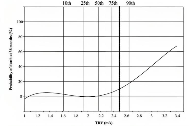
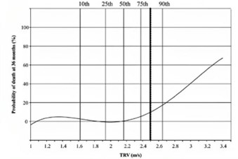
Tricuspid regurgitant jet velocity is considered a direct measurement of blood velocity returning from right ventricle to the right atrium during the systole according to Doppler echocardiography. This parameter is used for a
variety of purposes including right ventricular systolic pressure calculation (equivalent to the pulmonary artery systolic pressure). It can also be used as a measure of PH. For example, a value between 2.5 m/s and 3m/s identifies
25% to 39% of patients with a mean pulmonary pressure ≥ 25 mm Hg. In addition, it is linked to Lactate dehydrogenase (LDH) and plasma-free hemoglobin, which are known to be two biomarkers of intravascular hemolysis that may lead
to endothelial dysfunction and death within SCD patients
[23]
. Small fluctuations in the value of this parameter ≥ 2.5 are associated with an increased risk of mortality. A study published by Creteil (located in Paris) declared that TRV < 2.5 m/s is associated with less risk of death
compared to TRV values ≥ 2.5 m/s which is linked to a 6.81 mortality ratio.
[11]. Although SCD is common in sub-Saharan Africa, frequent high TRVs haven't been reported in Africa. Moreover, higher TRVs are associated with less 6-minute walk distance
[2].
Figure 5: The percentage of patients having 6-minute walk distance within various TRV intervals.
Figure 6: The relation between elevated TRVs and increased risk of mortality within a year
iii- Acute Splenic Sequestration Crisis (ASSC)
Acute Splenic Sequestration (ASS) is one of the most common complications of sickle cell anemia. Researchers define it as a drop in hemoglobin level with no less than 20%. This drop is related to an enlargement in spleen size by 2
cm at least compared with the patient's normal conditions
[26]
. The splenic sequestration starts with a blockage of splenic veins because of sickling blood cells in it resulting in occlusion. The blood entering the spleen is now normal and in good condition. However, the blood cells can't
exit the spleen well. These events can harm the circulatory system as it leads to hypovolemia and anemia [ 1]. In their first decade of life, sickle cell patients face ASS and specifically between five months and 2 years. Other
patients may face ASSC later in their life at about 8th decade
[26]
. In the crises, there are many reasons that make doctors determine if the patient has ASS or not. For example, sudden violation of anemia and splenomegaly, where the spleen becomes enlarged notability. In addition, on ASSC, the
bone marrow becomes active and after blood transfusion to the patient, the size of the spleen returns to the case before ASSC
[12]. There is another complication related to the spleen caused by sickle cell anemia called hypersplenism. But there is a difference between hypersplenism and Splenic Sequestration which is the fact that the spleen is always
enlarged in hypersplenism, and its size doesn't regress after blood transfusions
[1]. Depending on the level of riskiness, the attacks of ASS are separated into different types, which are minor attacks and major attacks. A moderate increase in spleen size and a quick decrease of the level of hemoglobin by 2—3
g/dl distinguish minor crises. While in major attacks the spleen size increases significantly, the anemia is greater than that of minor attacks as the level of hemoglobin reaches 2-3 g\dl, and it leads to hypovolemia. It is
thought that the cause of ASSC is associated with upper respiratory tract infection, and specifically, infection with human Parvovirus B19
[1]. ASSC diagnosis is done clinically, and complete blood count (CBC) is usually used to indicate the level of anemia, and reticulocytosis, in addition to white blood cells (WBC) and platelets as their level decreases
[12]. It is highly recommended to treat ASSC in a short time. Close monitoring and clinical evaluation should be done carefully. The intensive care unit (ICU) should keep the patients with major ASSC. Intravenous fluids should be
given to the patient in ASS. Patients also should be protected by giving them H. influenzae vaccines, meningococcal, and pneumococcal. Blood transfusion is usually used with ASSC patients. However, over-transferring can increase
blood viscosity. Blood viscosity may be greater as the stuck blood in the spleen can exit it and enter circulation after blood transfusion
[1]. It is important to measure the hemoglobin level after blood transfusion and keep it at its level before ASSC whatever it was
[12]. After one major attack, splenectomy is popular as the spleen becomes non- functional after that. In minor attacks, splenectomy is not highly recommended
[1], however, this step may be taken after two minor attacks
[12]. It is common to depend on chronic blood transfusion but that has its own risks. Blood-borne infections, iron overload, hepatitis, allosensitization, and others make blood transfusion not trusted
[1]. Although, on stopping blood transfusion, many patients will return to ASSC. So, the fact that splenectomy is recommended after two minor attacks is supported by the mortality rate of 20 %
[12].
V. Medications
i-Hydroxyurea
Hydroxyurea (HU) is the first U.S. Food and Drug Administration FDA-approved medication for sickle cell disease. By inhibiting the ribonucleotide reductase enzyme, this cytostatic agent drains the deoxyribonucleotide reserves
within the cells (used in DNA synthesis and repair). Also, this NO- releasing drug demonstrates a continuous inhibition of erythroid cell growth (reaching 20-40% within 6 days) and erythroleukemic K562 cell growth (reaching 65%
within 2 days)
[24]
. Its hematological consequences include elevated fetal hemoglobin level (a threshold of 20% is suggested to prevent recurrent Vaso occlusions), steady state hemoglobin level, and mean cell volume (MCV) as well
[27]
. On the other hand, a significant drop in the populations of leukocytes, reticulocytes, blood platelets, and hemolysis markers (bilirubin and LDH for example) is noticed
[19]
. Comparing the morphology of erythrocytes before enduring hydroxyurea therapy, the blood film shows significantly reduced intracellular cell sickling. The main principal mechanism of action of HU is thought to be augmented fetal
hemoglobin. Reduced leukocyte count caused by bone marrow suppression triggered by HU is expected to play an important role in Vasso- occlusion prevention as leukocytes are thought to be effective in VOCs initiation. The
Multicenter Study of Hydroxyurea (MSH) declared a 50% reduction in the annual rate of acute pain crises along with a significant drop in the rates of acute chest syndrome and blood transfusion requiring crisis in the patients on
which the study was carried out (HU was commenced at 15 mg/kg, this dose is elevated by 5 mg/kg/day to reach the maximum tolerated dose). Analogous outcomes were obtained from studies carried out on pediatric populations such as
the BABY-HUG study which included children aged between 9 and 18 months. prospective non- randomized studies imported improved organ function represented in the treatment of pulmonary hypertension, secondary stroke prevention,
lowered transcranial Doppler velocities, prevention of cerebral infarction, and preservation of splenic function
[28]
. For some of these, other studies couldn't reproduce these results. improvements including a reduction in life-threatening acute crises, less risk considering progressive organ damage, and improved life expectancy are noticed in
patients who adhere to the therapy in the long term and have good clinical and hematological responses. This is supported by the studies of each of the MSH, the Brazilian pediatric cohort, and the Laikon Hospital in Athens, Greece
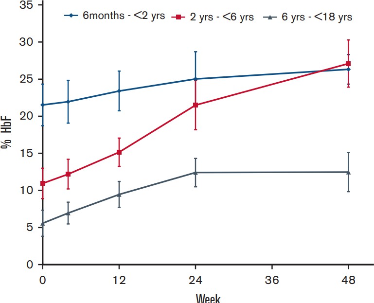
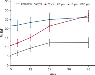
[12]. Another study conducted on 383 patients (59 died during the follow-up period) was designed to explain whether HU-induced HbF is associated with organ damage prevention and improved survival. The patients were assigned to four
quartiles depending on the maximum HbF. Only 71% of the patients in the lowest HbF quartile were alive, compared to 90% in the second quartile, 91% in the third quartile, and 86% in the highest one. The study also stated that
almost all of the patients in the highest quartile (97%) were assigned to the HU group (75% of the highest quartile patients were given the recommended doses), compared to only 33% in the lowest group (and only 18% were given the
recommended doses)
[9]. This is because HbF (α2γ2) lacks β-globin chains which provides it with anti- sickling effect in vitro by the interference with hemoglobin S polymerization
[5].
Figure 7: HU impact on HbF in patients of different ages.
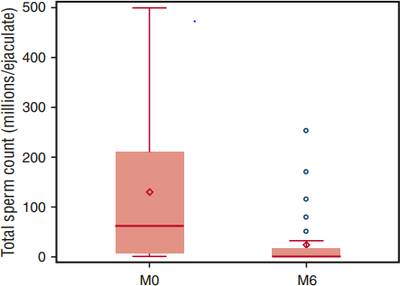
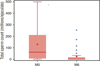
Figure 8: comparing the sperm count before and after 6 months of HU intake.
Unfortunately, some SCD complications don't show improvement and may even deteriorate more during HU therapy, including childhood avascular necrosis and priapism. Moreover, 25-30% of patients suffering from SCD have suboptimal
or no response at all to HU treatment
[14]. Furthermore, the HUSTLE trial reported long-term toxicities in children. Also, myelosuppression is a common HU adverse effect among patients intaking higher doses and older patients. To reduce its probability of occurrence,
the minimum effective dose is recommended. HU also has negative effects on spermatogenesis as it reduces sperm count and motility which normally don't return to normal even after giving off HU intake. Also, azoospermia was
reported in patients treated with HU
[4].
ii- Lentiviral Gene therapy
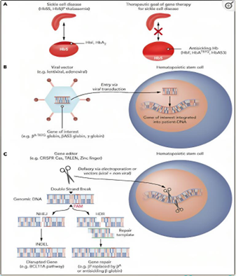
Contrary to the other SCD symptom-focused therapies, Gene therapy works to cure the disease itself. Unprecedented advances in genomic sequencing made the way for discoveries of new molecular tools for genome modification which
made gene therapy a promising medication for SCD. Though bone marrow transplantation and allogenic blood are known to cure SCD, donor availability restrictions (recent studies imported that less than 25% of patients found a
suitable intrafamilial donor) and graft-versus-host disease resemble significant drawbacks when they are compared to gene therapy
[31]
. Until now, only two techniques of gene therapy are known (gene adding and gene editing). Lentiviral gene therapy is among various gene addition therapies that use a variety of viral vector systems as lentiviral or adenoviral
vectors (due to their ability to introduce new genetic information into the living cells). Recently developed methods allowed the transfer of specific genes without viral replication which increases the potential of developing a
gene therapy for SCD. These gene modifications target hematopoietic stem cells (HSCs) (as they can be a life-long source of normal RBCs) and take place ex vivo in specialized facilities to avoid off-target genotoxicity that may
result from systemic delivery of viral vectors. These therapies aim to minimize the effect of βS either by producing normally functioning hemoglobin or anti-sickling hemoglobin. β-globin-based gene addition strategies work on
normal adult hemoglobin synthesis by incorporating and disappears during the first year of life. BCL11A is responsible for stopping γ-globin synthesis to switch to adult hemoglobin (HbA). After this, HbF represents only < 1% of
the total hemoglobin in erythrocytes. Patients with hereditary persistence of fetal hemoglobin (HPFH) along with SCD mutation have a mild SCD phenotype (due to reduced HbS concentration and HbF anti-sickling properties). Thus
γ-globin-based gene addition therapy targets increasing HbF by addition of γ-globin genes. Reversing the repression of γ-globin expression is considered an alternative. In lentiviral gene therapy, HSCs are harvested from the
patient, genetically modified ex vivo in cell culture, and then reinfused into the patient. To safely get through the harvesting procedure, patients are prepared through hydration and blood transfusions. Usually, patients undergo
several collection cycles to harvest enough cells for gene therapy. Lentiviral vectors (which are derived from HIV) precede all vector systems in gene addition strategies
[29]
. However, this thought was shaken by myeloid malignancies reported from patients following the therapy
[30]
. The genes of the virus used to obtain a lentiviral vector have been separated into individual plasmids. The lentiviral vector is obtained from transient expression of these plasmids and is loaded only with necessary genetic c
material needed to be transferred. Thus, it lacks the genes of replication and is self-inactivating due to a 3' long terminal cancellation. Because they incorporate into actively transcribed regions of the DNA, lentiviral vector
offers an advantage over retroviral vector which incorporates near gene regulatory regions
[32]
. β-globin genes into the DNA within the cell. The drawback concerning this strategy is leaving βS mutation intact, resulting in HbS still present in erythrocytes. The addition of anti-sickling gene variants is also under
development. This enables tracking the added gene expression. ΒA-T87Q and βAS3 are the two variants currently being discussed. Normally, γ-globin combines with α-globin to form HbF beginning in the third trimester of fetal
development.
Figure 9: Gene therapy techniques.
VIII. Conclusion
HbS is the main cause of SCD. Reducing HbS and/or its effects will manage SCD riskiness. It was found that blood transfusions can lead to many side effects making it not recommended by researchers in treating SCD. Hydroxyurea is
generally used to manage the complications and can't prevent all the disease. In addition, hydroxyurea can increase different disease complications while treating a specific complication. So, it was concluded that the smallest
functional dose of Hu is highly recommended than overusing it. On the other hand, gene therapy techniques can treat the disease itself and can help humanity end the crisis of sickle cell anemia. In addition, it is not a chronic
treatment, and patients will not need hospital visits after extracting enough hematopoietic stem cells to be gene- modified. Another key conclusion in gene therapy treatment is to use lentiviral, not retroviral, vectors to
increase the level of treatment in the therapy. So, the research question was answered by the fact that lentiviral gene therapy has a good potential to save SCD patients.
It is preferred to do future research to discover the hidden opportunities in lentiviral gene therapy to help poor patients as it is expensive nowadays. Hence, it may not be available in places like Africa where the disease
spreads and the health care levels are not high to enhance such a technique. That is noticed that economic aspects were not focused on in this paper.
IX. References
A Novel Framework in Leveraging Optimization Physics Models using Quantum Computing: Techniques for the 2-D Hubbard Model
Jefferson Lin (Northeast High School)
Mentor: Ahmed Ayman (El-Sadat STEM School)
Abstract
The new and emerging field of quantum computing harnesses the understanding of the complex dynamics of quantum systems, promising to advance and revolutionize scientific fields that can be applied in our world. However, realizing
this potential currently faces its challenges: scaling error-corrected qubits, parameter spaces, and efficiently compiling quantum circuits given hardware constraints. This paper reviews techniques to address these obstacles by
integrating automatically differentiable quantum circuits (ADQCs) with tensor networks (TN) to enable reverse-mode automatic differentiation for efficient optimization. We propose applying this ADQC-TN framework to the 2D Hubbard
model, which is a foundational model of strongly correlated electron systems exhibiting rich phase diagrams, including unconventional superconductivity. This framework can elucidate detailed mechanisms, such as how dopant atoms
influence superconducting electron pairing, by training the model's hopping, interaction, chemical potential, and other parameters on experimental measurements. Robust optimization represents a pivotal bridge between quantum
computing and experimental condensed matter physics to advance quantum-based materials modeling and discovery, which has already seen success from the extension of the ground state of quantum lattice models with low fidelities.
Successfully trained Hubbard models could facilitate the analysis and understanding of the effects of parameter-tuning and the potential of defects on superconductivity that can aid in other future modeling discoveries through
bridging the gap between quantum computing and physical engineering.
I. Introduction
When John Dalton first discovered the atom, a whole quantum world was waiting to be unveiled, a world where the principles of reality break down and what governs is beyond the naked eye. Based on these quantum mechanics, Feynman
and other scientists envisioned using quantum computers to simulate quantum systems under the premise that an initial quantum state can be unitarily evolved with a quantum computer that is polynomial in size and evolution time
[1]
. Such a potential, where a model Hamiltonian behavior could be simulated, became more than just an idea that physicists can use to broaden their understanding and determine what is intractable with classical, traditional
computers, from the smallest distances to cosmological extents
[2]
. Because classical computers are especially bad at simulating quantum dynamics in predicting how a highly entangled quantum state will change with time
[3]
, this newfound role of quantum computers in astronomically advanced modeling across physics, chemistry, and other domains
[4]
requires new tuning parameter methodologies to achieve more robust, scalable, and programmable methods in concurrence with technology application
[5]
. To match the new growing demands of limited hardware, costly simulations, being differentiable, challenging parameter spaces, and more, finding a way to optimize model parameters to match real measurements to have more accurate
models and simulations compared to experimental results is becoming a necessity as shown in Fig. 1.
Fig. 1. Illustration of classical computing and quantum computing structure with differing capabilities. Source:
[6]
Classical simulations of physical systems typically begin by solving differential equations, for the first order has the approximation $x(t+dt) \approx x(t) + f(x)dt$. However, when we try to simulate the microscopic world in
classical computers, the equations of motion are too complex as they are limited by conventional computing and classical physics. So, we must use quantum computing to simulate quantum systems. Through quantum computing (QC), a
complex quantum system can be isolated and controlled with sufficient precision to maintain quantum coherence
[7]
. We can manipulate these quantum states themselves, unlike classical computers, by implementing a universal set of quantum logic gates to approximate any unitary operation on the simulator’s qubits. Because Hilbert space grows
exponentially with system size $dim(H_{qubit})^{\otimes N}$, simulating quantum many-body dynamics on a classical computer becomes intractable. Quantum simulators can exploit effects such as entanglement, superposition, and
parallelism to encode and manipulate state space and operations compactly, allowing for massively parallel computation on the state vector, circumventing the limitations of classical simulation to develop quantum algorithms that
scale sub- exponentially in resources with the system size and desired accuracy. QC offers a computational advantage by meticulously using an exponentially ample Hilbert space for quiet registers (usually through sampling from
quantum states created by random entangling circuits) but is limited to specific tasks and problem 2 types. This advantage can be seen in molecular simulations with one such approach using Lie-Trotter-Suzuki product formulas
[8]
for Hamiltonian simulations, which reduces scalar error when each decomposition can be implemented into a quantum circuit. Similarly, recent developments in more optimal differentiable quantum generative models DQGMs
[9]
(on solving Fokker-Planck SDE equations) sampling enable the encoding of classical data into quantum states and the optimization of the quantum circuit parameters. All of this brings an essential discussion of using these quantum
systems to sample, solve efficiently, and model problems to reap the far-fetching benefits of QC in cryptography, simulations, optimization, and machine learning.
II. Quantum Physics
A. Schrödinger's Equation
In simulating quantum mechanics, we are first interested in the solution of the time-dependent Schrodinger equation,
$$ j\hbar \; \frac{\partial}{\partial t} |\; \psi(t)\rangle \; = \hat{H}|\psi(t)\rangle $$
(2.1.1)
where $H = -\frac{\hslash^2}{2m} \nabla^2 + V$ represents the Hamiltonian or the total energy of the wavefunction $\psi$ This can be further thought of as $\psi (t) = e^{-iHt} \psi (0)$ propagates the initial state $\psi (0)$ ‘s
evolution through time. The Schrodinger’s equation is a useful representation of quantum dynamics because it fundamentally describes how quantum systems evolve and their Eigen states, respectively. Additionally, it takes a
time-independent form $\hat{H} \psi = \hat{E} \psi$, but we will be focusing mainly on the time-dependent form and the applications resulting from it.
B. The Hamiltonian Approximation
The first idea is to approximate $\psi (t+ \Delta t)$ as $(I - iH\Delta t) \psi (t)$ like classical conventions, but, however, it is not satisfactory enough. We must turn to using the operator $e^{-i} \: \Delta t$ for $\psi (t +
\Delta t) = e^{-iH \Delta t} \psi (t)$ , under a sufficiently small-time step ∆𝑡 . For local Hamiltonians like Ising and Hubbard models, we can efficiently simulate by decomposing into smaller subsystems such that their complexity
is $O(polyN)$ , since applying $e^{-iHt}$ directly is expensive. For Hamiltonians like these as sub-Hamiltonians, it is first formulated by $H = \sum^b_a H_a .$ Then, we can apply the Trotter-Suzuki to approximate and decompose
the time evolution operator,
$$ e^{-iHt} =\; e^{-it} =\; \lim_{n \to \infty} \Biggl(\prod_{a}^{b}e^{-iHa\frac{t}{n}}\Biggl)^n $$
(2.2.2)
This simplifies to,
$$ \Biggl(\prod_{a}^{b} e^{-iHa\frac{t}{n}}\Biggl)^n \; + \; O \: \Biggl(\frac{b^2 t^2}{n}\Biggl) $$
(2.2.3)
The full Hamiltonian is decomposed into $b$ local terms $H_a$ with $e^{-iH_a t}$ representing its approximate evolution under the error $O (\frac{b^2 t^2}{n})$ For $n$ Trotter steps, there is a tradeoff to balance between accuracy
and efficiency because the error increases for more terms that do not commute $H{a_{1}} H{a_{2}} \ne H{a_{2}} H{a_{1}}$ under the time evolution $e^{-iH_a t} .$ So, in this first order error approximation, when $b$ increases, the
error increases as slowly as $n$ time steps is also increased respectively. This means that at the cost of more matrix multiplication, the accuracy improves. Let’s look at the Hubbard model as a simulation example
C. The Hubbard Model
The Hubbard model describes quantum tunneling as shown in Fig. 2 between neighboring lattice sites and on-site interaction between two fermions of opposite spin
[10]
. To construct our Hamiltonian, we can imagine a lattice of sites holding up to two electrons that can be spin up or down, hopping from one site to the next, written as
$$ \displaylines{ \hat{H}= \; - \sum_{ij} \sum_{\sigma} \: t_{ij}(\hat{a}^{\dagger}_{i \sigma} \hat{a}_{j \sigma} \: + h.c.) \; \\ + \frac{1}{2} \sum_{ijkl} \sum{\sigma \acute{\sigma}} \; \langle ij|v|kl \rangle
\hat{a}^{\dagger}_{i \sigma} \hat{a}^{\dagger}_{j \acute{\sigma}} \hat{a}_{l\acute{\sigma}} \hat{a}_{k\sigma}.} $$
(2.3.1)
where $t_{ij}$ is the hopping parameter between sites $i$ and $j$ , and $v$ the Coulomb potential. Under the two approximations of restricting hopping to only nearest neighbors and Coulomb interaction to only on-site
[11]
and adding a chemical potential term $\mu$, we have our second quantized 2-D Hubbard model,
$$ \displaylines{\hat{H}= \; -t \sum_{\langle i,j \rangle ,\sigma} (\hat{a}^{\dagger}_{i, \sigma} \hat{a}_{j, \sigma} \; \\ + \; \hat{a}^{\dagger}_{j, \sigma} \hat{a}_{i, \sigma}) + U \sum_{i} \hat{n}_{i, \uparrow} \hat{n}_{i,
\downarrow} \; - \; \mu \sum_{i,\sigma} \hat{n}_{i,\sigma} . }$$
(2.3.2)
Fig. 2. Illustration of 2-D cartoon quantum tunneling of Hubbard fermions. Source:
[12]
The first term represents the kinetic energy of electrons $t$ between neighboring sites $\langle i,j \rangle$ with a $a^{\dagger}_{i, \sigma}$ (creator) creating an election occupation at site $i$ with spin $\sigma$ and $a_{j,
\sigma}$ (annihilator) removing an electron occupation at site $j$ with spin $\sigma$ respectively. This is followed by the second term $U$ of the potential energy from the on-site Coulomb repulsion between electrons with opposite
spin using the number operator $n_{i, \sigma} = a^{\dagger}_{i, \sigma} a_{i, \sigma}$ for particles with spin $\sigma$ at site $i$ . The final term $\mu$ represents the chemical potential term needed when describing arbitrary
electron fillings, not just half-fillings, and affects the total number of particles. When half-filling, the Hubbard model exhibits a Mott metal-insulator transition, taking the system from a metal to an antiferromagnetic
insulator. Beyond the Mott transition, the Hubbard model provides insights into diverse broken symmetry phases and phase transitions in strongly correlated systems. The competition parameters $\frac{U}{t}$ between the potential
energy term $U$ that favors localization and insulating behavior and the kinetic energy term $t$ that favors delocalization and metallic behavior, alongside the chemical potential $\mu$, give rise to the rich physics of magnetism
and superconductivity. This framework of quantum lattices is widely believed to contain the essential ingredients of high-temperature superconductivity because of its delicate competition between the parameters. Doping of charge
strips and superconductivity turned by parameter t′ has shown the prediction of a Luther-Emery (LE) liquid that demonstrates a close interplay between charge and superconductor correlations
[13]
. The Hubbard model thus serves as a simplified theoretical foundation for understanding complex interacting quantum materials. However, the model’s simplicity is deceptive as it is a mathematically difficult problem to solve due
to its many-body nature, with an exact solution only found in the 1D case
[14]
. A simple example of this model is to consider a system with just two sites,
$$ \psi=|n_{1 \uparrow} n_{1 \downarrow} \rangle | n_{2 \uparrow} n_{2 \downarrow} \rangle $$
(2.3.3)
having $2^4$ possible states depending on the kinetic energy determining how the initial filled each lattice is. This state of an isolated quantum system with $n$ components is represented by a state vector in a Hilbert space of
dimension $2^n$ possible states for $n$ qubits with each qubit able to be in a superposition of 0 and 1 . If we want to simulate the dynamics of a quantum system by discretizing time into steps of length $\Delta t$ at each time
step, we need to multiply the state vector by the propagator matrix corresponding to evolving the system for a time ∆𝑡. Therefore, the propagator matrix has dimensions $2^n \times 2^n$ with the computation cost scaling as $O(2^n
\times 2^n)$ (see Fig. 3). For most cases, this exponential scaling makes the exact simulation of quantum systems with even 50 − 100 qubits completely impractical on classical computers due to the exponential growth of the
operator that leads to the discussion of using optimization techniques.
Fig. 3. Demonstration of Big-O complexities. Our goal is to find a low computational cost towards the bottom of the graph. Source:
[15]
III. Quantum Computing
A. Jordan Wigner-Mapping
To utilize quantum computing, we must transform the Hamiltonian into a set of operations accessible or understandable to quantum computers. Namely, we can use the simple Jordan Wigner transformation for second quantized
Hamiltonians to map occupations to qubit orientations, simulating fermionic systems on qubits and gates by using Pauli-$X$ and -$Y$ to satisfy $a^{\dagger}_{i} | 0 \rangle_{i} = 0, a_{i} | 1 \rangle_{i} = 0,$ and $a^{\dagger}_{i}
| 1 \rangle_i = 0,$
$$ a^{\dagger}_{i} = \frac{X_i - i Y_i}{2}, a_i = \frac{X_i + i Y_i}{2} . $$
(3.1.2)
Fig. 4. Illustration of state preparation and mapping of models with the intermediate step of transformation. Source:
[16]
For this mapping to capture the antisymmetric characteristics of fermions $a^{\dagger}_{i} a_j = -a^{\dagger}_{j} a_i,$ we must intersperse Pauli-$Z$ to remedy the fact that Pauli Operators do not commute for $XY \ne -YX,$ but
rather for $XZ = -ZX$ and $YZ = -ZY$:
$$ \displaylines{ a^{\dagger}_{1} = \frac{X_1 - i Y_1}{2} \; \Huge\oplus \normalsize 1 \Huge\oplus \normalsize 1 \; ... \Huge\oplus \normalsize 1 \\ a^{\dagger}_{2} = Z_1 \Huge\oplus \normalsize \frac{X_2 - i Y_2}{2} \;
\Huge\oplus \normalsize 1 \Huge\oplus \normalsize 1 \; ... \Huge\oplus \normalsize 1 \\ a^{\dagger}_{n} = Z_1 \Huge\oplus \normalsize Z_2 \Huge\oplus \normalsize ... \Huge\oplus \normalsize \frac{X_n - Y_n}{2} . } $$
(3.1.3)
We get,
$$ X_i Y_i = i Z_i \newline \therefore n_i = a^{\dagger}_i a_i = \frac{1-Z_i}{2} . $$
(3.1.4)
Over the Jordan-Wigner transformation, the Hubbard Hamiltonian in equation (2.3.2) becomes
$$ \displaylines{ H = -\frac{t}{2} \sum_{\langle i,j \rangle} Z_{j+1:i-1} (X_i X_j + Y_i Y_j) + \\ \frac{U}{4} \sum_i (1-Z_i^{\uparrow})(1-Z_i^{\uparrow}) - \frac{\mu}{2} \sum_{i, \sigma} (1-Z_i^{\sigma}) . } $$
(3.1.5)
Other mappings include the Bravyi-Kitaev
[17]
, Parity, and those that can perform more advanced qubit reductions available in quantum computing softwares like Qiskit
[18]
. From this transformation, we can break down the Hamiltonian into two terms such that $H = H_0 + H_1,$ where $H_0$ is the kinetic term, and $H_1$ the other two interaction terms. Then, by applying the Trotter-Suzuki
decomposition, we get
$$ e^{-iHt} = \lim_{n \rightarrow \infty}(e^{-iH_0 \frac{t}{n}} e^{-iH_1 \frac{t}{n}})^n . $$
(3.1.6)
This allows us to approximate the time evolution operator by breaking up the evolution into successive n short time steps and repeating while taking larger n improves the accuracy of the approximation. However, we can begin to see
the complexities and computational cost arising from higher-order approximations. The natural instinct from this is try to find optimization techniques to circumvent this.
B. Tensor Network Optimization
Now that we can convert our Hamiltonian into quantum computing language, we must face the fundamental problem of optimizing a quantum circuit: efficiently exploiting parameters. We can solve this through differentiable programming
given hardware constraints by minimizing the loss function that encodes the problem we want to solve,
$$ \alpha_{t+1} = \alpha_t \; - \eta \nabla_\alpha \mathcal{L} (\alpha, t) $$
(3.2.1)
where $\alpha$ are the parameters, $\eta$ the learning rate, and $\nabla \mathcal{L}$ the gradient operator on the loss function. This loss function can be largely responsible for the feedback on how well a quantum circuit is
performing given a set of parameters, updating it each time for optimization, and is commonly used in machine learning. We can use tensor networks (TN), useful mathematical, graphical representations of multi-dimensional arrays
that can store information through tensor nodes in a computation graph. We can significantly enhance optimization by exploiting automatic differentiation in the tensor computation graph. This technique of backpropagation exploits
the chain rule of a partial differential to propagate the gradient back from the network output and calculate the gradient of the weight respectively
[19]
. With the forward pass being
$$ |\psi\rangle=U(\alpha)|\psi_0\rangle \newline \langle O \rangle = \langle \psi |O|\psi \rangle $$
(3.2.2)
where $U(\alpha)$ representing a quantum circuit with parameters $\alpha$ acting on initial state $| \psi_0 \rangle$ to produce output state $| \psi \rangle$ , followed by the expectation value of $O$ , a physical observable that
could be represented by a Hermitian operator. We can begin to see the similarities with the original system quantum evolution representation for application,
$$ \psi(t)=e^{-iHt} \psi(0). $$
(3.2.3)
From this, the implications of applying backpropagation through the expectation value computation to get gradients with respect to circuit parameters tying to the simulation of quantum systems are obvious. After this forward pass,
we can backpropagate (backwards pass) this through the chain rule and see the loss function $L$ depending on the expectation value $\langle O \rangle$,
$$ \frac{\partial L}{\partial \alpha} = \frac{\partial L}{\partial \langle O \rangle} = \frac{\partial \langle O \rangle}{\partial \alpha} $$
(3.2.4)
Representing this in tensor networks through the traversing of data flow as in nodes, we can visually see the chain rule and reverse-mode automatic differentiation
[20]
,
$$ \displaylines{ \alpha \rightarrow W^1 \rightarrow W^2 \ldots W^n \rightarrow L \newline \frac{\partial L}{\partial \alpha} = \frac{\partial L}{\partial W^n} \frac{\partial W}{\partial W^{n-1}} \ldots \frac{\partial
W^1}{\partial \alpha}. \newline \leftarrow \leftarrow \leftarrow \leftarrow \leftarrow \leftarrow \leftarrow } $$
(3.2.5)
Fig. 5. Illustration of tensor networks through backpropagation to minimize a loss function. The transaction channels can be represented by multiple tensors that can split off respectively depending on intended algorithms that
are widely applicable in machine learning. We can also visually see the backpointing technique in storing checkpoints. Our single $\alpha$ tensor network serves as a fundamental representation in equation (3.2.5). Source:
[21]
We can also see that the resulting relationship of $O$ relating to physically meaningful observable and arbitrary intermediate tensor $W$ are analogous in the role they play. In order to reduce memory usage, we can employ the
backpointing technique, conceptually like checkpointing (see Fig. 5), where one can simply store the tensor every few steps in the main node. Relying on differentiating through these tensor networks has shown state-of-the-art
calculations of specific heat of the Ising model, variational energy, and magnetization of the antiferromagnetic Heisenberg model
[20]
as an efficient compression of quantum states.
C. Automatically Differentiable Quantum Circuits Tensor Networks (ADQC-TN)
Now that we have discussed optimization, how can we leverage these tensor networks and automatically differentiate them in quantum circuits? We have the tools of TN to simulate quantum models with ample Hilbert space through the
backpropagation technique to reduce complexity, but what do we do with them? The simple answer is reframing our thinking to apply to quantum circuits.
Remember our goal is to simulate a model onto quantum circuits,
$$ |\psi_{tar}=I(\alpha)|\psi_{evol}\rangle $$
(3.3.1)
where $| \psi_{tar} \rangle$ is the target state evolved from operation $U(\alpha)$ on $| \psi_{evol} \rangle$ state. We want to minimize the error between the target and evolved state,
$$ F=-\frac{1}{N}\ln | \langle \psi_{tar} | U(\alpha)|\psi_{evol}\rangle| $$
(3.3.2)
where $F$ is the negative logarithmic fidelity that quantifies the closeness between the $| \psi_{tar} \rangle$ and $| \psi_{evol} \rangle$ states over operation $U(\alpha)$ . Therefore, we just need to find a particular set of
unitary gates or operations on $\delta^*$ parameters that minimizes $F$ , our respective loss function. This can be done by updating the gates towards the opposite direction of their gradients and integrated with TN
[22]
,
$$ \displaylines{ \delta^{\boldsymbol{\cdot}} = U \Lambda V^{\dagger} \newline \delta^{\boldsymbol{\cdot}} \leftarrow \delta^{\boldsymbol{\cdot}}_0 - \eta \frac{\partial F}{\partial \delta^{\boldsymbol{\cdot}}} } $$
(3.3.3)
where $\delta^{\cdot}$ projects to a set of unitary gate $\delta^*$ under $Tr(\delta^{\cdot} \delta)$ to be maximized from constraint $\delta$ . This is then fed into the backpropagation integrated with TN. All we have to do after
is apply our desired Hamiltonian into this system and compare it with traditional methods
IV. Applications
A. Variational Quantum Eigensolver (VQE)
One current, powerful application is the Variational Quantum Eigensolver (VQE)
[23]
, a hybrid quantum-classical algorithm to find a Hamiltonian’s minimum eigenvalue and eigenstate. VQE aims to minimize energy by optimizing a set of parameters $\alpha$ for a chosen ansatz quantum circuit. The circuit has two
purposes: prepare the ansatz wave function $| \psi (\alpha) \rangle$ and measure the expectation value $\langle \psi (\alpha) | H | | \psi (\alpha) \rangle$ which gives the energy. A classical optimizer uses this measurement to
adjust $\alpha$ to lower the energy toward the true ground state. Starting with initial parameters $| \psi (\alpha_0)\rangle = e^{-iH | \psi (\alpha_0) \rangle} | \psi_1 \rangle$ the ansatz circuit prepares the trial wavefunction,
where $| psi_1 \rangle$ is a simple starting state. In variational quantum algorithms like VQE, the loss function is typically the expectation value and minimizing the loss, we find the ground state energy. Measuring the
expectation energy $E(\alpha_0)$ provides an upper bound on the true ground state energy:
$$ E(\alpha_0) = \langle\psi(\alpha_0)|H|\psi (\alpha_0)\rangle \ge E_0 $$
(4.1.1)
The classical optimizer then generates new parameters $\alpha_1,$ using $E(\alpha_0)$ to guide it closer to the minimum. This optimization loop of state preparation, measurement, and classical processing repeats until converging
on an ansatz $| \psi (a^*) \rangle$ that minimizes $E(\alpha) \approx E_0$ .This hybrid quantum algorithm is useful for quantum chemistry and optimization problems that looks analogous to the issues we can solve with ADTNAQCs. VQE
implementations on existing quantum hardware are limited by qubit error rates, the number of qubits available, and the allowable gate depth
[24]
, and new techniques implementing better optimization methods and representation of these compact spaces like ADQCs and TNs are necessary for the continued further application of quantum computing despite quantum hardware
restrictions as shown in Fig. 6.
Fig. 6. Illustration of the application of quantum computing for manipulating data sets. We can visually see here the usage of optimization techniques and programming for a desired output, dependent on the algorithm. Source:
[25]
B. Modeling
The advent of Automatically Differentiable Quantum Circuits (ADQCs) allows for preparing many-qubit target quantum states by optimizing gates through differentiable programming via backpropagation. ADQCs introduce unconstrained,
differentiable latent gates projected to unitary gates satisfying quantum constraints, and therefore optimizing these latent gates layer-by-layer yields efficient state preparation using ADQCs, obtains low fidelities, and can
reduce matrix product state (MPS) representations with a compression ratio of $r \sim O(10^{-3})$
[22]
. Likewise, tensor networks are a powerful mathematical tool that can provide a compact representation of high-dimensional quantum states and quantum many-body physics
[26][27]
by formulating tensor networks as differentiable computation graphs. A key advantage is directly computing tensor network output gradients, enabling the evaluation of observables. This yields optimal performance for infinite 2D
tensor networks and finding the ground states of lattice models
[20]
. When integrated with ADQCs, TN can demonstrate intelligent quantum circuit construction combining machine learning techniques, a promising approach for training and optimizing quantum systems using modern differentiable
programming. Such applications can already be seen in the development of built-in ADQC programs such as Yao
[28]
, which can optimize a variational circuit with 10,000 layers using reverse-mode AD and constructing 20 sites Heisenberg Hamiltonian in approximately 5 seconds. By utilizing this paper's framework and quantum computing softwares,
one can model and optimize their desired models.
V. Future Research
There are two main sectors of future research from ADQC-TN optimization on models: other physical models and applicable optimization. Future research into non-local Hamiltonians and other respective techniques and approximations
extends to models beyond the 2D Hubbard model. Similarly, higher dimensions and more complex, accurate models are good starting points. Having a framework to see which methods apply to what, so that it can be tailored for real
applications, would be branching out. The frame-work proposed for optimizing parameters in this paper relies mainly on quantum computing software. The work in more advanced and enhanced libraries and programing could determine
usability, automation, utilization, and integration into real-world systems. New loss functions, flexible architectures, and alternative quiet mappings, in combination with more methodological and pragmatic engineering fronts,
will aid in the discovery and application of accurate, performant quantum models. Furthermore, future research can also be seen in real-world applications of the techniques discussed in this paper. The integration of machine
learning methods with automatic differentiation and tensor networks using quantum circuits can help in model tuning, complex algorithms, and optimization in the fields of artificial intelligence and quantum simulation. This can
already be seen in
[29]
, where hybrid neural network weight tensorization can be represented by a tensor-train data format to compress parameters that developed an energy-efficient machine learning accelerator. More motivation can be seen in
[30]
for the intellectual combination of tensor networks and neural networks for potential applications in information fusion and more specifically, what neural networks has already seen development like natural language processing and
robotics can be improved.
VI. Discussion
Further technical examination of this ADQC-TN approach can reveal several aspects of the modeled Hamiltonian and optimization as a field. Firstly, alternative transformations such as the Bravyi-Kitaev algorithm offer potential for
more efficient reductions that could reduce overall circuit depth, and more detailed analysis quantitatively comparing circuit complexity under different fermionic qubit mappings could in advantageous transformations for a given
model. Secondly, this tensor network architecture design space is extensive and dependent heavily on depth, entanglement, connectivity, and the desired model. Architectures balancing expressiveness and trainability may be
particularly well-suited, but systematic evaluation of tensor network configurations' usage will be essential in creating performant models applicable beyond physical domains. Thirdly, while mathematically convenient, reliance on
fidelity as the sole optimization metric is not ideal and is best alongside incorporating alternative domain-specific loss functions for training towards precise experimental objectives under a given objective. Fourthly, while
simplified, differentiable programming is still in its infancy and requires more development on its widespread software, meaning modeling difficulty and complexity will depend similarly on the software used.
This paper lays a framework for optimizing the 2-D Hubbard Hamiltonian model implementable in quantum programming languages. For other models alike, it can be done in three simplistic steps: This paper lays out a framework for
optimizing the 2-D Hubbard Hamiltonian model implementable in quantum programming languages. For other models alike, it can be done in three simplistic steps:
Integrate our desired Hamiltonian model and utilize any unique simplifications and/or approximations in equation (2.3.2).
Transform that Hamiltonian to qubit (QC) language via the desired transformation seen in equation (3.1.5).
Apply an optimization method to find the desired output and/or parameters of the Hamiltonian model using equation (3.3.3).
VII. Conclusion
Pursuing a simplified framework in leveraging optimization and programming techniques that can be used to transition from theoretical quantum physics to applied quantum computing is essential in further understanding the promising
use of new quantum simulation methods and integration of quantum hybrid methods over just classical simulations. This paper has proposed a framework for optimizing parameters of the 2D Hubbard model by integrating automatically
differentiable quantum circuits with tensor networks. We reviewed techniques for gradient- based optimization via backpropagation through ADQCs to enable efficient tuning of quantum circuits. The Hubbard model was transformed into
qubit operators using the Jordan-Wigner transformation to implement on a quantum circuit. By minimizing the fidelity error between target and evolved states, the ADQC-TN framework can optimize model parameters to match
experimental measurements. The proposed ADQC-TN optimization framework for simulating the 2D Hubbard model offers a path forward despite hardware constraints. As quantum computing matures, techniques like differentiable
programming will help implement precise quantum models to revolutionize our understanding of complex quantum materials. New research into complex quantum systems and their applications in quantum computing is necessary for the
diversity of software and paradigms. Techniques alike leverage what is already known but make it better and more applicable to reduce problems from new growing demands like computational complexity costly simulations, and is
scalable, to name a few. By outlining a methodology of the potential application of automatic differentiation using tensor networks in models like the Hubbard model, this paper summarizes the problems faced and current, novel
solutions to it. This can go beyond simulating just local models and be more applicable to other parameters in increasing complexity. As the times of our technology try to catch up, looking from a different perspective and way of
thinking will help in the endeavor to make sense of and apply these innovations despite the limitations of our time.
VIII. References
D. Wecker, M. B. Hastings, N. Wiebe, B. K. Clark, C. Nayak, and M. Troyer, "Solving strongly correlated electron models on a quantum computer," Phys. Rev. A, vol. 92, no. 6, pp. 062318, Dec. 2015, doi:
10.1103/PhysRevA.92.062318.
C. W. Bauer et al., "Quantum Simulation for High Energy Physics," arXiv, Apr. 07, 2022, doi: 10.48550/arXiv.2204.03381.
J. Preskill, "Quantum Computing in the NISQ era and beyond," Quantum, vol. 2, pp. 79, Aug. 2018, doi: 10.22331/q-2018-08-06-79.
M. Reiher, N. Wiebe, K. M. Svore, D. Wecker, and M. Troyer, "Elucidating reaction mechanisms on quantum computers," Proc. Natl. Acad. Sci. U.S.A., vol. 114, no. 29, pp. 7555—7560, Jul. 2017, doi: 10.1073/pnas.1619152114.
J. Fraxanet, T. Salamon, and M. Lewenstein, "The Coming Decades of Quantum Simulation," 2022, doi: 10.48550/ARXIV.2204.08905.
C. W. Bauer et al., "Quantum Simulation for High Energy Physics," PRX Quantum, vol. 4, no. 2, p. 027001, May 2023, doi: 10.1103/PRXQuantum.4.027001.
Q. Liu, "Comparisons of Conventional Computing and Quantum Computing Approaches," HSET, vol. 38, pp. 502—507, Mar. 2023, doi: 10.54097/hset.v38i.5875.
O. Kyriienko, A. E. Paine, and V. E. Elfving, "Protocols for Trainable and Differentiable Quantum Generative Modelling," arXiv, Feb. 16, 2022. Accessed: Aug. 21, 2023. doi. 10.48550/arXiv.2202.08253.
E. Cocchi et al., "Equation of State of the Two-Dimensional Hubbard Model," Phys. Rev. Lett., vol. 116, no. 17, p. 175301, Apr. 2016, doi: 10.1103/PhysRevLett.116.175301.
V. Celebonovic, "The two-dimensional Hubbard model: a theoretical tool for molecular electronics," J. Phys.: Conf. Ser., vol. 253, p. 012004, Nov. 2010, doi: 10.1088/1742-6596/253/1/012004.
C. Miles et al., "Correlator convolutional neural networks as an interpretable architecture for image-like quantum matter data," Nat Commun, vol. 12, no. 1, p. 3905, Jun. 2021, doi: 10.1038/s41467-021-23952- w.
H.-C. Jiang and T. P. Devereaux, "Superconductivity in the doped Hubbard model and its interplay with next-nearest hopping t'," Science, vol. 365, no. 6460, pp. 1424—1428, Sep. 2019, doi: 10.1126/science.aal5304.
X.-W. Guan, "Algebraic Bethe ansatz for the one-dimensional Hubbard model with open boundaries," J. Phys. A: Math. Gen., vol. 33, no. 30, pp. 5391—5404, Aug. 2000, doi: 10.1088/0305-4470/33/30/309.
J. W. Z. Lau, K. H. Lim, H. Shrotriya, and L. B. Kwek, "NISQ computing: where are we and where do we go?," AAPPS Bull., vol. 32, no. 1, p. 27, Sep. 2022, doi: 10.1007/s43673-022-00058-z.
A. Tranter, P. J. Love, F. Mintert, and P. V. Coveney, "A Comparison of the Bravyi— Kitaev and Jordan—Wigner Transformations for the Quantum Simulation of Quantum Chemistry," J. Chem. Theory Comput., vol. 14, no. 11, pp.
5617—5630, Nov. 2018, doi: 10.1021/acs.jctc.8b00450.
M. Watabe, K. Shiba, M. Sogabe, K. Sakamoto, and T. Sogabe, "Quantum Circuit Parameters Learning with Gradient Descent Using Backpropagation," 2019, doi: 10.48550/ARXIV.1910.14266.
H.-J. Liao, J.-G. Liu, L. Wang, and T. Xiang, "Differentiable Programming Tensor Networks," Phys. Rev. X, vol. 9, no. 3, p. 031041, Sep. 2019, doi: 10.1103/PhysRevX.9.031041.
P.-F. Zhou, R. Hong, and S.-J. Ran, "Automatically Differentiable Quantum Circuit for Many-qubit State Preparation," 2021, doi: 10.48550/ARXIV.2104.14949.
J. Tilly et al., "The Variational Quantum Eigensolver: a review of methods and best practices," 2021, doi: 10.48550/ARXIV.2111.05176.
J. M. Clary, E. B. Jones, D. Vigil-Fowler, C. Chang, and P. Graf, "Exploring the scaling limitations of the variational quantum eigensolver with the bond dissociation of hydride diatomic molecules," Int J of Quantum
Chemistry, vol. 123, no. 11, p. e27097, Jun. 2023, doi: 10.1002/qua.27097.
S. Raubitzek and K. Mallinger, "On the Applicability of Quantum Machine Learning," Entropy, vol. 25, no. 7, p. 992, Jun. 2023, doi: 10.3390/e25070992.
R. Orus, "A Practical Introduction to Tensor Networks: Matrix Product States and Projected Entangled Pair States," 2013, doi: 10.48550/ARXIV.1306.2164.
R. Orus, "Tensor networks for complex quantum systems," 2018, doi: 10.48550/ARXIV.1812.04011.
X.-Z. Luo, J.-G. Liu, P. Zhang, and L. Wang, "Yao.jl: Extensible, Efficient Framework for Quantum Algorithm Design," 2019, doi: 10.48550/ARXIV.1912.10877.
H. Huang, L. Ni, and H. Yu, "LTNN: An energy efficient machine learning accelerator on 3D CMOSRRAM for layer- wise tensorized neural network," in 2017 30th IEEE International System-on-Chip Conference (SOCC), Munich: IEEE,
Sep. 2017, pp. 280—285. doi: 10.1109/SOCC.2017.8226058.
M. Wang, Y. Pan, Z. Xu, X. Yang, G. Li, and A. Cichocki, "Tensor Networks Meet Neural Net-works: A Survey and Future Perspectives," 2023, doi: 10.48550/ARXIV.2302.09019.
A quantitative study: How inflammatory diet affects different neurotransmitters' function and their relation to memory disorders.
Abdelrahman Gamal (Ismailia STEM high school)
Adam Hassan (Fayoum STEM high school) Karim Morgan (Gharbiya STEM high school) Mentor: Habiba Sorour
Abstract
Alzheimer's disease has been a case study for a long time, discoveries brought hypotheses and reasons related to the disease mechanism. This study aims to bring a clear understanding of the significant impact of human actions such
as diet and Alzheimer's disease. Diet indirectly impacts the human body and significantly the brain, in the case of memory disorder diet affects the neurotransmitters that play an important role in the function of the brain and
memory. The study used various relations between variables, hypotheses show that a transmembrane protein plays a key role in neurodegeneration and later it disturbs the neurotransmitter's function. Through the study, information
showed that diet styles cause oxidative stress which is considered one of the main reasons that cause neurodegeneration. The study shows the impact of each variable on the other and leads these findings to the main case study of
Alzheimer's disease.
I. Introduction
The brain is an Extortionary organ as it is responsible for thoughts, memories, and movement of the body systems and function, furthermore, the brain health acquires attention and care. Due to the brain's vulnerability to some
disorders. cognitive brain disorders occur due to the detectable destruction of brain connections or networks between neurons, and neurodegenerative diseases such as Alzheimer's disease (AD), Parkinson's Disease (PD),
Schizophrenia, Depression, and Multiple Sclerosis (MD). Some of these disorders are mainly caused by the imbalance of the neurotransmitter levels or the disturbance in its function. Neurotransmitters are basically messengers,
molecules in the nervous system are used to transmit messages between neurons through synapses.
Alzheimer's disease is a cognitive disorder, where About 55 million people have dementia, and %60 of this population has Alzheimer's disease. The onset stage of this disease is memory loss, and in later stages, the patients could
have problems with speaking, eating, and swallowing or the disability to walk.
Yet the neurological disorders in some cases of its distributions are in some point revolve around human actions and habits such as diet and how it could increase the chances of Alzheimer's disease development. This paper will
focus on contributing relations and mechanisms in terms of represented information on the impact of diet on Alzheimer's disease and presenting relations between different variables that have an important role in the study,
variables due to diet impact such as oxidative stress others belong to Alzheimer's disease causes such as amyloid beta, and acetylcholine. The study contributes to the relationship between these variables and their significant
role in the case of Alzheimer's disease and diet.
i. Inflammatory Diet
The body's natural, important defense against microbial infections, tissue damage, and trauma is called inflammation. It supports the body's ability to recover from injury and protect itself. Inflammation promotes the immune
response by enlisting innate immune cells that are capable of producing inflammatory cytokines (i.e., signaling proteins). Particularly, the innate immune system of the body is under the control of the gene transcription factor
kappaB (NF-κB). However, Inflammation can be harmful if it persists for a long time. When (NF-κB) is continuously activated as a result of consuming inflammatory food, inflammation becomes chronic. Chronic inflammation causes a
dysregulated immune response, which disturbs physiological functions that are meant to be homeostatic.
Inflammation hugely contribute to causing diseases such as inflammatory bowel disease (IBD), [diabetes mellitus], [asthma], cardiovascular diseases, [depression,] Alzheimer's disease (AD), and different types of cancer[1]Inflammatory and anti-inflammatory foods: Diet can influence different stages of inflammation. Inflammation can result from being exposed to environmental toxins, aging, or chronic stress.
On one hand, the over consuming of inflammatory foods can cause inflammation, including red meat, processed meat, snack cakes, pies, cookies and brownies, bread and pasta made with white flour, deep-fried items — French fries and
fried chicken —, and high-sugar food — such as candy, jelly, syrup, soda, bottled or canned tea drinks, and sports drinks.
On the other hand, healthy eating patterns help put inflammation down and stay healthier. These patterns can be achieved through being committed to consuming particular types of supplements found in food, including Omega-3 — found
in different types of fish, nuts, and seeds-, Vitamin C — found in fruits and vegetables —, and polyphenols — found in the wise consuming of tea, coffee, and dark chocolate.[2]
ii. Neurotransmitters
Mechanism: Neurotransmitters are the nervous system's way of delivering messages to the rest of body organs and parts through nerve cells. Each neurotransmitter is responsible for a function, which may be moving a certain muscle,
activating memory or appetite, controlling blood pressure, .... etc.
[3]
They are also involved in the processes of early human development, including neurotransmission, differentiation, the growth of neurons, and the development of neural circuitry
[9]
. Certain neurotransmitters may appear at different points of development. For example, monoamines, neurotransmitters responsible for controlling basic emotions and affecting major depressive disorders, are present before the
neurons are differentiated
[9]
.
At presynaptic nerve terminals, neurotransmitters are primarily released via vesicular action. Neurotransmitters are released into the synaptic cleft mainly via calcium-evoked exocytosis of presynaptic vesicles. The
neurotransmitter- containing vesicles are attached to the plasma membrane by active zones, specialized regions on the presynaptic plasma membranes. Action potentials cause calcium to enter the presynaptic cleft, which causes the
active zones to fuse with the vesicles and release neurotransmitters. The fusion of neurotransmitter-containing vesicles and the active zone is mediated by several proteins. The exocytosis of neurotransmitters from the presynapse
may be inhibited and activated as well by these proteins; Synaptobrevin-2, SNAP-25, and syntaxin-1 collectively make up the soluble N-ethylmaleimide sensitive factor attachment protein receptors (SNAREs), which are essential for
membrane fusion and ultimately exocytosis.
[4]Acetylcholine and Serotonin: The neurotransmitter acetylcholine (ACh) is primarily responsible for memory-related processes. Furthermore, it is crucial for cognitive, memory, and learning processes in brain nerve
cells. It moves voluntary muscle, muscle movement you control, all over the human body by binding to muscarinic receptors. It also regulates heart contractions and blood pressure, lowers heart rate, moves food by contracting
intestinal muscles, increases stomach and intestine secretions, causes glands to secrete substances like tears, saliva, milk, sweat, and digestive juices, regulates the flow of urine, and contracts muscles that control nephrons.
On the other hand, it causes skeletal muscle to contract by binding to nicotinic receptors, which releases adrenaline and norepinephrine from the adrenal glands, activating the sympathetic nervous system in humans.
[5]
Serotonin, also referred to as 5- hydroxytryptamine (5-HT), is a monoamine neurotransmitter. In addition to its hormone-like properties, it plays a part in morphogenesis, the biological process by which both body structure and
form emerge during embryonic development. It also has a significant impact on a number of other bodily processes, such as mood regulation (when serotonin levels are normal, you feel more alert, emotionally stable, happier, and
calmer, and vice versa), regulating sleep (along with dopamine, serotonin helps the brain regulate how well and how long a person sleeps), wound healing (serotonin narrows blood vessels, which slows blood flow and causes clots to
form), and bone density (high levels of serotonin lead to weak bones and vice versa).
[6]
iii. Alzheimer's disease
Alzheimer's disease is a progressive brain disorder that deteriorates with time, characterized by significant changes in the brain due to the accumulation of certain protein deposits. This process ultimately leads to brain atrophy
and, in some cases, brain cell death
[13]
. Gradual decline in memory, cognitive abilities, and social skills is a hallmark of Alzheimer's, making it the leading cause of dementia
[13]
.
In the United States, approximately 6.5 million individuals aged 65 and older live with Alzheimer's disease, with more than 70% of them being 75 years or older
[14]
. Globally, of the roughly 55 million people living with dementia, an estimated 60% to 70% are believed to be affected by Alzheimer's disease
[14]
.
On a global scale, the year 2020 witnessed over 55 million individuals grappling with dementia. According to data from Alzheimer's Disease International (ADI), the number of people afflicted with dementia has nearly doubled
approximately every two decades
[14]
.
The primary symptom associated with Alzheimer's is memory loss. In its early stages, individuals with the disease may recognize their struggles with memory recall and clear thinking. Alzheimer's-induced changes in the brain
progressively lead to challenges in six key areas: memory, cognitive abilities, decision-making, planning and executing tasks, behavioral shifts, and the loss of fundamental skills
[12]
.
However, according to (ADI) research, the majority of people who are now living with dementia have not received a formal diagnosis. Only 20-50% of dementia cases are recognized and documented in primary care in high-income nations
[14]
. This treatment gap is undoubtedly considerably wider in low and middle-income nations, with one research in India claiming that 90% of patients go misdiagnosed
[14]
. If these figures are extrapolated to other nations, it appears that almost three-quarters of people with dementia have not been diagnosed, and hence do not have access to the treatment, care, and organized support that a formal
diagnosis may bring. Alzheimer's disease patients typically live between three and eleven years after diagnosis
[14]
. However, some people survive for 20 years or more
[13]
. The degree of disability at the time of diagnosis can have an impact on life expectancy
[13]
. Untreated vascular risk factors, such as hypertension, are linked to a higher rate of Alzheimer's disease progression
[12]
.
Alzheimer's disease is classified into five detailed stages:
The first stage: Preclinical Alzheimer's disease: During this time, neither the patient nor those around them will notice any symptoms
[12]
. This stage of Alzheimer's can last for years, possibly even decades. New technologies can identify the tangles development, which develop when tau proteins change shape and organize into structures. These are hallmarks of
Alzheimer's disease
[12]
.
Additional biomarkers for Alzheimer's disease have been discovered. These are present in blood tests and may suggest a higher risk of disease
[12]
. These biomarkers can be used to help confirm an Alzheimer's disease diagnosis, usually after symptoms develop
[12]
. Newer imaging techniques, biomarkers and genetic tests will become more important as new treatments for Alzheimer's disease are developed
[13]
.
Second stage: Mild cognitive impairment due to Alzheimer's disease: Mild cognitive impairment causes minor deficits in memory and thinking skills
[12]
. These modifications aren't large enough to have an impact on job or relationships
[12]
. Memory lapses may occur in people with MCI when it comes to knowledge that is normally easily remembered
[12]
. This could include recent discussions, activities, or appointments.
Individuals with Mild Cognitive Impairment (MCI) may also encounter challenges in gauging the time needed for various activities. Estimating the number or sequence of steps required to complete a task can become problematic, and
making well-informed decisions might grow more challenging
[12]
.
It's important to note that not everyone with MCI progresses to Alzheimer's disease. Typically, MCI is diagnosed based on a thorough assessment of symptoms and the clinical judgment of healthcare professionals. However, if
necessary, the same diagnostic tests employed to identify early-stage Alzheimer's disease can also be used to ascertain whether MCI is a result of Alzheimer's disease or another underlying cause.
Moving on to the third stage: Mild dementia attributed to Alzheimer's disease. Alzheimer's disease is often recognized during the initial phases of mild dementia. At this point, both family members and medical professionals
observe significant difficulties in memory and cognitive reasoning
[12]
. These symptoms notably impede everyday functioning.
This stage of detecting memory loss of recent activities, trouble with problem solving and sound judgment, changing personality, and getting lost or misplacing belongings
[12]
.
Fourth stage: Moderate dementia due to Alzheimer's disease: People get more confused and forgetful during the moderate dementia stage of Alzheimer's disease. They begin to require more assistance with daily activities and
self-care
[13]
.
Fifth stage: Severe dementia due to Alzheimer's disease: It is the late stage of Alzheimer's disease, where mental function continues to decline. The disease is also having an increasing impact on movement and physical capacities
[12]
.
Patients in this stage lose the ability to communicate, and experience a decline in physical abilities, for instance, they cannot walk without assistance
[12]
. Moreover, they require daily assistance and personal care
[13]
.
II. Methods
The study contributes the different relation between variables and how these variables impact each other to better understand the mechanism of Alzheimer disease, with a clear understanding of these relations, the study could
demonstrate the significant impact of diet on Alzheimer's Disease. The aim connection is between diet and Alzheimer's Disease, the variable relation is the connection dots which start with Amyloid- β as the key role in Alzheimer's
disease pathogenesis and considering the role of the neurotransmitters. On the other side of the study, the diet has various styles with each having its significance though this study contributes the diet styles that have a
significant correlation with Alzheimer's disease, in terms of the diet styles such as vegetarian diet that cause oxidative stress which is responsible for the inflammation and neurodegenerative disorders in the neurons. The
significant contribution is the experimental data of the vegetarian diet food and its impact on disturbing vitamins and mineral levels in the body, in that matter, vitamins deficiency such as vitamin B12 and vitamin D that
vegetarian diet food lack, these vitamins absent or deficiency could increase the risk of Alzheimer's disease.
(I) Role of Amyloid- β in Alzheimer's disease pathogenesis
Figure 1: represent the stages of APP cleavage in the neuron membrane
Amyloid β (Aβ) is considered a critical reason for the development of Alzheimer's disease (AD) the senile plaques (SPs) and intracellular neurofibrillary tangles (NFTs), which results in the loss of neurons and synapses. The SPs
are formed by aggregation of (Aβ) as some studies propose that it is a small protein composite of 39-43 amino acids
[18]
.
At (B) phase in Figure 1: represents the two cleavage processes of Amyloid precursor protein (APP), it is a transmembrane glycoprotein with a large luminal domain and a short cytoplasmic domain. In processing of
cleaving the (APP) and Aβ formation, APP could go through either an amyloidogenic or non-amyloidogenic pathway
[18]
.
The amyloidogenic pathway is the process of Aβ formation, in this pathway APP is firstly cut by β-secretase, producing soluble β-APP fragments (APPβ) and a C-terminal β fragment (C99), C99 is further cut by γ-secretase, generating
APP intracellular domain (AICD) and Aβ as a non-soluble fragment
[3]
.
The non-amyloidogenic pathway is another way to prevent the formation of Aβ, as APP is firstly cut by α-secretase within the Aβ domain, producing soluble α-APP fragments (APPα) and C-terminal fragment α (C83), C83 is then cleaved
by γ-secretase
[3]
.
i. Biochemistry of Amyloid β-Protein and Amyloid Deposits in Alzheimer's Disease
Figure 2: code sequence of amyloid plaques
Amyloid (A) is a 39-43 residue amyloidogenic peptide that is deposited in the extracellular amyloid plaques
[6]
, whose 1-letter code sequence is shown in Figure 2. That defines the brain of people with Alzheimer's disease (AD). On chromosome 21, there is the gene for amyloid beta precursor protein. Moreover, it is formed
by the enzymatic cleavage of APP, the Amyloid Precursor Protein, a type-1 transmembrane protein produced in many organs, particularly the central nervous system (CNS)
[6]
.
Figure 3: microscopy image of a neurotic (senile) plaque in the cortex of an Alzheimer's patient
According to some studies on modern research on the fundamental mechanism of Alzheimer's disease (AD). The meningovascular amyloid subunit in Down's syndrome brains was the same "β-protein," as they had dubbed it. Glenner drew
attention to this evidence of a crucial biochemical link between Down's syndrome and AD, a theory he had championed in a foresighted paper in Medical Hypotheses as early as 1979 (Glenner 1979)
[15]
. Glenner reasoned that since trisomy 21 caused an accumulation of Alzheimer-type A in arteries and plaques, familial AD may well be caused by a deficiency in the -protein precursor on this chromosome. Glenner omitted to mention
the variability of familial types of AD and the possibility that many cases may not be genetically determined, at least at the time.
Figure 3 represents a Confocal microscopy image of a neurotic (senile) plaque in the cortex of an Alzheimer's patient that has been three- dimensionally rebuilt. Amyloid -protein is colored red by an antibody to
identify extracellular amyloid, and tau is colored green by an antibody to reveal closely related dystrophic neurites. The plaque core, it should be noted, is not a single, porous mass of amyloid, but rather is broken up and
contains aberrant cell processes intercalated therein
[8]
.
ii. Amyloid beta and acetylcholine
Figure 4: Aβ and cholinergic transmissionFigure 4 shows the Targets of Aβ that modulate cholinergic transmission:
(1) Aβ reduces the activity of pyruvate dehydrogenase, an enzyme that generates acetyl coenzyme A (CoA) from pyruvate, (2) Aβ reduces high-affinity uptake of choline; (3) long-term or high-dose exposure to Aβ reduces activity of
the choline acetyltransferase (ChAT) enzyme; (4) Aβ reduces acetylcholine (ACh) content; (5) Aβ reduces ACh release from synaptic vesicles (SV); (6) Aβ impairs muscarinic M1-like signaling. AChE = acetylcholinesterase, Ch U =
site of choline uptake, M2 = presynaptic muscarinic M2 receptor, N = presynaptic nicotinic receptor, PtdCho = phosphatidylcholine.[16]
The studies of APP and Aβ
[17]
, suggest the notion that overexpression levels of Aβ peptide, and the aggregation of Aβ that cause subcellular alterations or neuronal loss in selected brain regions. The great levels of Aβ peptide may incentivize the formation
of neurofibrillary tangles in tau in some experiments on mice[18]
. Furthermore, these results suggest that Aβ peptides have a role in the neurodegenerative process in which the nerve cell loses its function and dies.
Degeneration of neurons and synapses in the brain along with AD, could be located within regions that contain high levels of plaques and tangles
[17]
. Regions include the hippocampus, entorhinal cortex, amygdala, neocortex, and basal forebrain cholinergic neurons, Biochemical investigations indicated that there are neurotransmitters including acetylcholine (ACh), serotonin,
noradrenaline, and somatostatin, as they are differently related with AD
[4]
.
The findings include a reduction in the activity of the ACh-synthesizing enzyme, and choline acetyltransferase (ChAT)
[17]
, in the neocortex, which correlates with dementia. Reduced choline absorption, and ACh loss of cholinergic neurons from the basal forebrain region it was hypothesized that is due to the inactivity of acetylcholine could cause a
cholinergic deficit in the hippocampus and neocortex of brains of those with AD and these cholinergic neurons is either spared or affected in the late stages of the AD[17]
.
Basal forebrain cholinergic neurons loss has led to the study of ACh receptors in the brains of AD patients. ACh affects the central nervous system by interacting with G-protein-coupled muscarinic and ligand-gated cation channel
nicotinic receptors. Five distinct muscarinic receptor subtypes, m1—m5. Studies suggest that AD patients have a decrease in muscarinic receptors in their brains.
III. Results
i. Vegetarian diet lack of vitamins associated with AD.
The vegetarian diet is a diet style based on consuming plant-based food, however, this diet style may be beneficial in many aspects but it was noticed that this type of diet may increase the risk of some cognitive diseases such as
Alzheimer's disease, due to the plant-based food lack of some essential vitamins such as vitamin D and vitamin B12.
Vitamin B12, are essential water-soluble micronutrients that have to be consumed in sufficient quantities in the diet. They are necessary for preserving hematopoiesis and the health of neurons
[11]
. In affluent nations, vitamin B12 insufficiency is uncommon, although it is widespread and affects 10 to 15% of people over the age of 60 and 25 to 35% of people over the age of 80
[11]
. The antioxidative property of vitamin B12, with B12 deficiency, might lead to the oxidation of lipids, proteins, and nucleic acids and so it could contribute to the development of age-related diseases, in which oxidative stress
is a major factor, including AD
[10]
, and Parkinson's disease.
In which the different processes that were explored on how vitamin B12's antioxidant effects work, including direct scavenging of ROS, particularly superoxide in the cytosol and mitochondria, and indirectly increasing ROS
scavenging via maintaining glutathione levels
[10]
. Additionally, vitamin B12 may offer defense against oxidative damage brought on by inflammation. Vitamin B12 reduction is associated with an increase in interleukin-6 production and TNF-α levels. Interleukin-6 has a role in
inducing hyperphosphorylation of tau and TNF-α increases the Aβ burden by upregulating β-secretase production and increased γ-secretase activity
[10]
.
A study was done on 15 different groups
[11]
, with the objective of finding a positive result on vitamin B12 deficiency and the increase in oxidative stress. This study is a collection of different scientists' studies on this topic, the data were based on experiments from
different countries in India, Egypt, Romania, Turkey, Italy, Oman, and Jordan.
These studies were based on some common terms of vitamin B12 markers and oxidative stress biomarkers such as MDA, GSH, TAC, TAS, and SOD that basically support increased oxidative stress or reduced antioxidant capacity in case of
lower B12 status.
In these data there were different study cases of the 15 groups: there were two retrospective studies (RS), two cross-sectional studies (CS), and seven case- control studies (CC). Figure 5: the Number of studies that overall support, do not support, or show unclear results regarding the antioxidant properties of B12, in total and per study type.
Figure 6: Number of statistical tests for all study types for common oxidative stress biomarkers that significantly (p < 0.05) support increased oxidative stress or reduced antioxidant capacity in case of lower B12 status.
The study results showed that the majority of the experiments contribute to the main objective.
Nine out of 15 studies supported the antioxidant properties of B12 (60%). One did not (6.7%). Five showed unclear results (33.3%). As shown in Figure 5[11]
.
Five CC studies, one CS, one RS, and two animal studies supported B12 as an antioxidant. Notably, the potential antioxidant effect of B12 was unclear for both RCTs due to their broad-spectrum micronutrient interventions. As shown
in
Figure 6
[11]
.
IV. Discussion
Oxidative stress is a condition caused by an imbalance between production and accumulation of oxygen reactive species (ROS), including superoxide radicals (O2), hydrogen peroxide (H2O2), hydroxyl radicals (OH), and singlet oxygen
(^1^O2), in cells and tissues and the ability of a biological system to detoxify these reactive products. The majority of ROS are produced by mitochondria. Cellular respiration, the lipoxygenases (LOX) and cyclooxygenases (COX)
involved in the metabolism of arachidonic acid, as well as endothelial and inflammatory cells, can all produce O2
[5]
.
Environmental stressors, including UV, ionizing radiation, pollutants, heavy metals, and anti- stress medications also contribute to increasing ROS levels, which lead to the occurrence of oxidative stress. Numerous diseases,
including Parkinson's disease, Alzheimer's disease (AD), amyotrophic lateral sclerosis (ALS), multiple sclerosis, depression, and memory loss, have been linked to oxidative stress; oxidative stress plays a role in the loss of
neurons and development of dementia in Alzheimer's. The toxic peptide _β_-amyloid, which is produced by free radical action and frequently found in the brains of AD patients, is at least partially responsible for the
neurodegeneration seen during the onset and progression of AD
[11]
.
ii. Oxidative stress and the amyloid beta peptide in Alzheimer's disease
Figure 7: shows the detailed process of the oxidative damage.
Oxidative stress is known to play an important role in the pathogenesis of a number of diseases
[7]
. It is specifically associated with the etiology of Alzheimer's disease (AD), an age-related neurodegenerative illness that is the leading cause of dementia in the elderly. Furthermore, AD is characterized by intracellular
neurofibrillary tangles and extracellular production of senile plaques formed of aggregated amyloid-beta peptide (A) and metal ions such as copper, iron, or zinc
[5][6]
.
Active metal ions, for example, copper, can speed up the production of Reactive Oxygen Species (ROS) when bound to the amyloid-β (Aβ). Thus, ROS can be produced in the hydroxyl radical, which is the most reactive one, which may
lead to oxidative damage on both the Aβ peptide and surrounding molecules (proteins, lipids, etc. )
[7]
.
Given the importance of oxygen, the many systems for producing and eliminating ROS, and their regulation, it is not surprising that oxidative stress has been linked to a wide range of disorders. Furthermore, oxidative stress can
become a vicious cycle, as the created ROS can degrade biomolecules, leading to further ROS accumulation. For example, when ROS attack metalloproteins, they can cause the release of redox-competent metal ions, leading to an
increase in ROS production. Additionally, the brains of people suffering from neurodegenerative disorders such as Alzheimer's and Parkinson's reveal oxidative damage, and oxidative stress appears to be a factor in many of them.
Because the brain consumes so much dioxygen (20% of total body consumption), it may be especially vulnerable to oxidative damage under oxidative stress
[6]
.
Apart from the global reduction in the brain volume, one of the hallmarks of Alzheimer's disease is the existence of amyloid plaques in the brain, which is caused by the "deposition of a special substance in the cortex," as first
described by Alos Alzheimer. These plaques, also known as senile plaques, are seen in the extracellular space of the AD brain, notably in the hippocampus. They are predominantly made up of a peptide called Amyloid- (A), which
aggregates and produces mostly -sheet rich fibrils. The existence of intracellular neurofibrillary tangles in the brain
[3]
, which are also seen in Parkinson's disease (PD) and are made up of hyperphosphorylated Tau protein, is another feature of the disease. To stabilize microtubules, this microtubule-associated protein typically interacts with
tubulin.
Metal ions such as zinc, iron, and copper are found in the brain, as previously stated. They are required to modulate neuronal activity in synapses and are engaged in metallo-protein biological processes. Metal ion homeostasis is
impaired in various illnesses, including Alzheimer's, and concentrations and distribution are far from normal. Cu and Zn levels, in particular, can reach up to three times the typical levels found in healthy brains. Furthermore,
amyloid plaques isolated from AD brains contain a significant concentration of these metal ions. Because they can bind to A at physiological concentrations, their coordination modalities are of interest in understanding their
function in Alzheimer's disease
[6]
.
ROS are radicals and molecules formed when molecular oxygen is incompletely reduced. They are created in modest amounts during the in vivo metabolism of oxygen, via four sequential 1-electron reductions of O2 that result in the
creation of H2O. They are required for cell homeostasis and play a crucial role in signaling, but they are also reactive oxidants that can damage biomolecules
[6]
.
iii. Oxidative stress and diet
Reactive Oxygen Species (ROS) and Reactive Nitrogen Species (RNS), which are involved in metabolism, development, and stress response, are essentially what produce oxidative stress. This unbalanced state may cause oxidative damage
by oxidative modification of cellular macromolecules, structural tissue damage from cell death via necrosis or apoptosis, and cell death via apoptosis. ROS are highly reactive molecules with unpaired electrons that can affect how
biological processes work. Proteins, lipids, and nucleic acids may undergo structural and functional damage as a result of oxidative stress.
Oxidative stress is basically caused by mitochondria via oxidative phosphorylation that generates intracellular ROS. Meanwhile, ROS causes a mitochondrial malfunction. The NADPH oxidase family (NOX) and oxidative phosphorylation
in mitochondria are the main sources of H2O2. For an organism to remain in a healthy state, the proper ROS are required. However, excessive ROS has been linked to a variety of health issues, such as obesity, cancer, cardiovascular
disease, and neurological illnesses.
Cognitive diseases such as Parkinson's disease and Alzheimer's disease are examples of neurodegenerative diseases that affect the elderly. They are characterized by a progressive loss of neuron cells and diminished mobility or
cognitive function. Mitochondrial dysfunction is one of these disorders' key traits. To supply the energy requirements for cellular functions, particularly the synthesis of neurotransmitters and synaptic plasticity, the
mitochondria in neurons have a crucial role. Increased mitochondrial permeability, mitochondrial disorganization, oxidative damage to mtDNA, weakened antioxidant defenses, and shortening of telomeres are all associated with
mitochondrial dysfunction. Due to their high energy needs, high fatty acid content, high mitochondrial density, and low bioavailability of antioxidant compounds and antioxidant therapy, neurons are particularly vulnerable to
oxidative stress. In Alzheimer's disease, Aβ aggregation causes Ca2+ release from the endoplasmic reticulum to the cytoplasm, which could lead to a decrease in the accumulation of ROS. Neuronal functions are impaired, which
further leads to neuroinflammation and neuronal loss.
Diet can control mitochondrial disease. A study found that patients with Lennox-Gastaut syndrome (LGS), a common form of refractory epilepsy, with mitochondrial dysfunction, experienced a significant clinical improvement in both
seizures and cognitive performance. Patients with heart failure benefit from taking more docosahexaenoic acid (DHA), an n-3 polyunsaturated fatty acid. By binding to membrane phospholipids, lowering the viscosity of mitochondrial
membranes, and speeding up the uptake of Ca2+, DHA supplementation can enhance the DHA content in mitochondrial phospholipids, preventing the onset of left ventricular failure.
Unpaired electrons are produced by cells during regular cellular respiration as well as under stressful conditions, usually via oxygen- or nitrogen- based byproducts. These highly unstable pro-oxidant compounds have the potential
to oxidize nearby biological macromolecules. Over time, the development and buildup of reactive pro-oxidant species can harm lipids, carbohydrates, proteins, and nucleic acids. This oxidative stress has the potential to exacerbate
a number of age-related degenerative disorders, including Alzheimer's and Parkinson's.
There are various diet styles and one of the most common diet styles is the Western diet, which is considered by the high intake of saturated fats, highly refined carbohydrates, and animal-based protein and a deficiency in the
consumption of plant- based fiber. It has been shown that people who eat a Western diet food are more likely to develop chronic disease and have higher levels of oxidative stress. In the Western diet style, consuming too much fat
causes oxidative stress, mitochondrial damage, and inflammation. High-calorie diets disrupt redox processes, accelerating aging signs and raising the risk of chronic diseases.
Antioxidants that include vitamins, and minerals can counteract this oxidative damage as they play a role in protecting the cell from free radicals such as ROS and RNS. Therefore, diet plays a crucial role in health, via specific
food consumption that could disturb antioxidant levels in the body, therefore affecting cellular function and disease risk, emphasizing the importance of balanced nutrition and lifestyle interventions.
V. Conclusion
In conclusion, this research adds to our understanding of the complex interactions between nutrition, inflammation, neurotransmitters, and oxidative stress in Alzheimer's disease. It underlines the importance of dietary and
lifestyle changes in lowering the risk of Alzheimer's disease and lays the groundwork for future research into targeted therapeutics. As we continue to learn more about the complexity of neurodegenerative disorders, a multifaceted
strategy that includes nutrition, neurobiology, and oxidative stress management may hold the key to a better future for people at risk of Alzheimer's disease.
Our research has revealed numerous crucial findings, offering light on prospective routes for additional investigation and therapeutic approaches. Our findings highlight the significant role of nutrition in the development and
progression of Alzheimer's disease. We've discovered that an inflammatory diet high in processed foods, red meats, sweet desserts, and high-sugar beverages promotes chronic inflammation, a known cause of AD. In contrast, we've
highlighted the protective potential of anti-inflammatory foods like Omega-3 fatty acids, vitamins, and polyphenols, which may reduce the risk of AD.
Amyloid-β (Aβ), a key player in AD pathogenesis, has been explored in the context of its interactions with neurotransmitters and oxidative stress. Our findings suggest that Aβ accumulation can disrupt cholinergic and serotonergic
neurotransmission, contributing to cognitive decline. Moreover, the interplay between Aβ, metal ions, and oxidative stress may accelerate neurodegeneration.
Oxidative stress emerges as a common denominator linking inflammatory diets, neurotransmitter dysregulation, and Aβ toxicity in Alzheimer's disease. The Overproduction of reactive oxygen and nitrogen species (ROS and RNS) causes
cellular damage, notably in mitochondria, and contributes to neurodegenerative processes. Managing oxidative stress by food and antioxidants may provide therapeutic benefits.
Our findings highlight the possibility of dietary treatments in reducing the risk and course of Alzheimer's disease. Individuals who follow an anti- inflammatory diet may reduce chronic inflammation, support neurotransmitter
balance, and combat oxidative stress, boosting brain health and memory preservation.
VI. Refernces
A comparison: galactic formation & evolution through semi-analytic and numerical hydrodynamic frameworks in the context of extragalactic astronomy.
Malak Elsaied (Gharbiya STEM High School)
George Salib (STEM High School for boys 6th of October)
Abstract
In our never-ending cosmic quest to understand the origin of the universe, galactic evolution is profound, as galaxies make up a considerable portion of our universe. Additionally, understanding galactic evolution and the
phenomena involved will provide us with the necessary foundation to make predictions about the fate of galaxies and our Milky Way. Although many advances have been made in the field of cosmology, our knowledge of galactic
formation and evolution still possesses key gaps. To understand galactic evolution, cosmologists design models of the universe and simulate galactic evolution under the effects of dark matter, dark energy, and baryonic matter. In
this article, we mainly discussed two types of frameworks used in designing galactic simulation models: the semi-analytic and numerical hydrodynamic frameworks; we also talked briefly about the N-body and Lamda Cold Dark Matter
frameworks. Numerical hydrodynamic simulations provide a tool for investigating the complex and dynamic interactions between numerous physical processes. Meanwhile, semi-analytic models use analytical approximation techniques to
handle a range of variables. When choosing a simulation model, the computational complexity of the hydrodynamics framework and the uncertainty of the semi-analytic models prove to be a conundrum. So, we have discussed both
frameworks, comparing their advantages and limitations. We concluded that currently both frameworks complete each other's shortcomings, and for a superior understanding of galactic formation and evolution, a more comprehensive
framework that combines both approaches is needed.
I. Introduction
There is still a lack of knowledge regarding the mechanisms that led to the formation and evolution of the earliest galaxies, following the Big Bang. Understanding the mechanisms underlying their formation and evolution is crucial
to understanding how galaxies will develop in the future. According to previous research
[1][2][3][4][5], models have been created to aid in the attempt to comprehend and study the processes of galaxy formation through cosmologicalsimulations. The numerical hydrodynamic simulations and semi-analytic models are derived from these
frameworks. Both have widespread use, and each has advantages and disadvantages. Given the enormous number of variables involved, numerical hydrodynamic simulations offer a tool to explore the intricate and dynamic interplay
between many physical processes. While semi-analytic models use approximation analytical methods to cope with a variety of variables. The physical processes of galaxy creation and evolution, several models used to represent these
processes, numerical hydrodynamics simulations, semi-analytical models, and examples for both models are included in this review article.
II. The Physical Processes of Formation and
The models used to comprehend and implement the formation and evolution of galaxies mostly include the physical processes covered in this section.
i. Gravity
The first galaxies are thought to begin as small clouds of dust and stars, and as other clouds come near them, gravity ties them together. The cosmological parameters and the characteristics of dark matter affect the shape and
magnitude of the primordial power spectrum of density fluctuations. The number of dark matter halos of a particular mass that have collapsed at any given moment can be calculated from this spectrum, which is processed by gravity
to determine how quickly these halos expand throughout cosmic time through merging and accretion
[6]. It also controls the spatial organization of dark matter halo clusters. According to the conventional theory, each galaxy is born within one of these "shadowy" haloes. Gravitation and dynamical friction progressively drive the
orbits to decay until the galaxies combine in halos that each contain their central galaxy. Mergers can have significant impacts on galaxies, including causing bursts of star formation and accretion onto supermassive black holes
at the center, as well as changing the structure and appearance of the galaxy
[6].
ii. Hydrodynamics and Thermal Evolution
Intense shocks are created during the collapse of an excessively dense province made of gas and dark matter, which raises the entropy of the gas. The gas's ability to reflect thermal energy away and cool down successfully will
then decide how the gas evolves in the future. Two-body radiative processes are the main cooling mechanisms important for galaxy formation during most of cosmic history. At a temperature of more than 10than 10^7^ Kelvin, gas
becomes entirely collisionally ionized and cools mostly through bremsstrahlung (free-free emission)
[6]. Collisionally ionized atoms can return to their ground state and electrons can join with ions in the temperature range of 10^4^ K to 10^7^ K. The collisional excitation/deexcitation of heavy metals (metal line cooling) and
molecular cooling are the two processes that cause cooling below 10^4^ K. If radiative cooling is ineffective after collapse and shock-heating, a pressure-supported quasi- hydrostatic gaseous halo may develop. Then, in a process
that is commonly referred to as a cooling flow, this gas will progressively cool. A different name for this is "hot mode" accretion
[6]. The gas will collapse until it is supported by its angular momentum once it cools and loses pressure support. Without ever producing a hot quasi-hydrostatic halo, the gas may accrete straight onto the proto galaxy if the
cooling time of the gas is short relative to the dynamical period
[7]. According to cosmological hydrodynamic simulations, gas tends to flow along relatively cold, dense filaments during this type of "cold mode" accretion
[6].
iii. Star Formation
Once the gas has condensed into the halo's central regions, it may start to self-gravitate or be driven more by its gravity than by dark matter. If cooling processes prevail overheating, then a runaway process can occur in which
Giant Molecular Cloud (GMC) complexes form, and eventually some dense cloud cores within these complexes collapse and reach the extreme densities required to ignite nuclear fusion. This is because gas cools more quickly the higher
its density, so if cooling processes dominate, then a run-away process can occur
[6]. Many aspects of this process are still unclear, though. According to observations
[8][9], 1% of molecular gas turns into stars every period of free fall, which is a practically universal efficiency for star formation
[10]. The gas is often transformed into star particles using a probabilistic sampling approach based on a calculated star formation rate
[10]. Many cosmological simulations are unable to distinguish between individual cores, much less the scales on which GMC emerges. Therefore, to describe star formation, all current cosmological simulations use empirical sub-grid
recipes. Since cold, dense gas eventually gives rise to stars, simulations convert a portion of this gas into collisionless star particles, which reflect coeval, single-metallicity stellar populations that are characterized by an
underlying initial stellar mass function
[10]. A few simulations additionally take star clusters into account as the primary unit of star formation by enabling the expansion of star particles through accretion from the surrounding medium. This is an alternative to the
probabilistic sampling strategy and helps to better mimic the clustered nature of star formation. Modern galaxy formation models track stellar evolution and the mass return of these stars to the gas component after stellar
particles have been generated.
iv. Star Formation Feedback
Less than 10% of the current global baryon budget, according to observations, is in the form of stars. We would anticipate that most of the gas would have cooled and generated stars by the present day in Cold Dark Matter (CDM)
models without any sort of "feedback" (or suppression of cooling and star formation). This "overcooling problem" was acknowledged even by the forerunners of the earliest models of galaxy formation within a CDM framework, who
hypothesized that the energy from supernova explosions may heat gas and possibly blow it out of galaxies, impeding star formation
[6]. It is now understood that a variety of processes, like photo-heating, photoionization, and winds, that are connected to massive stars and supernovae may have a role in star formation inefficiency and large-scale winds that
lower galaxies' baryon fractions. Again, the majority of cosmological simulations are unable to resolve these physical processes in detail. Therefore, almost all the current models use sub-grid recipes to try to simulate their
impact on galaxy scales
[6].
v. Black Hole Formation and Growth
As the remains of Population III (metal-free) stars, through the direct collapse of extremely low angular momentum gas or stellar dynamical processes, the first black holes may have formed in the early universe
[11]. These black holes can expand by either absorbing gas with very little angular momentum or by generating an accretion disk that drains the gas's angular momentum through viscosity. These processes are modeled via sub-grid
recipes since they are, once more, poorly understood and nearly hard to model explicitly in cosmological simulations
[6]. The most likely scenario is that the black holes develop at high redshifts as the remains of the first generation of Population III stars have passed their prime. It is still unclear how exactly these first stars formed, but
hydrodynamical simulations indicate that they had masses of about a few hundred Solar masses and left behind intermediate-mass black hole remnants
[12].
Cosmological black holes have an additional characteristic, angular momentum, in addition to their mass. Essentially, merging with another black hole and material accretion are the two processes that alter a black hole's spin
[12].
vi. Active Galactic Nuclei (AGN) Feedback
Strong observational evidence suggests that a supermassive black hole is present in most spheroid- dominated galaxies, which make up most of all big galaxies. A straightforward calculation shows that the energy released in
creating these black holes must be greater than the host galaxy's binding energy, indicating that it could have a significant impact on galaxy formation. However, how effectively this energy can couple to the gas in and around
galaxies is still unknown
[6]. High-velocity winds, which may be expelling the cold interstellar medium from galaxies, and hot bubbles that appear to be produced by enormous radio jets, which may be heating the hot halo gas, are two observational indicators
of feedback linked with AGN. In modern cosmological simulations, AGN feedback is also handled with sub- grid recipes
[6]. Active galactic nuclei relate to observational phenomena related to accreting supermassive black holes, including electromagnetic radiation, relativistic jets, and less-collimated non- relativistic outflows
[10]. Quasar and radio modes, which are used differentially in simulations, are the two most prevalent divisions of this feedback. Some galaxy formation models, however, claim that cosmological simulations lack the resolution
necessary to accurately distinguish between the two feedback modes and to keep the number of feedback channels to the minimum necessary to match the observational data. These models do not make this distinction
[10]. The radiatively efficient mode of black hole growth is linked to quasar mode feedback, which is frequently implemented through energy or momentum injection under the assumption that the bolometric luminosity corresponds to the
accretion rate and that a fixed portion of this luminosity is deposited into the nearby gas
[10]. Radio-mode feedback occurs by highly collimated jets of relativistic particles, which are frequently coupled with X-ray bubbles containing enough energy to compensate for cooling losses. This feedback mechanism is therefore
thought to be crucial for controlling star formation in large galaxies. As soon as the accretion rate drops below a threshold level, radio-mode feedback is frequently incorporated as a second subresolution feedback channel
[10]. The subresolution models for supermassive black holes are still unclear considering that they must cross a gap between real accretion and feedback and the scales that can be defined with simulations
[10].
vii. Stellar Populations and Chemical Evolution
Many modelers convolve their predicted star formation histories with straightforward stellar population models that provide the Ultraviolet — Near Infrared Spectral Energy Distribution for stellar populations of a single age and
metallicity
[13], folding in an assumed stellar Initial Mass Function to directly compare models and observations
[6]. In many models nowadays, gas recycling from star mass loss is considered in simulations in a significant way. It is also clear that stars pollute the intergalactic medium out to great distances from galaxies as they develop and
undergo supernovae, producing and dispersing heavy metals throughout the gas that surrounds galaxies
[6]. Due to several factors, including (1) the highly enhanced cooling rates at intermediate temperatures in metal-enriched gas, (2) the metallicity-sensitive luminosity and color of stellar populations of a given age, and (3) the
production of dust by heavy elements, which dims and reddens galaxies in the UV and optical and re- radiates the absorbed energy in the mid-to-far IR, chemical evolution is a crucial component of galaxy formation. The treatment of
chemical evolution is currently present in many cosmological models of galaxy formation
[6].
viii. Radiative Transfer
Star and AGN radiation can have a significant effect on galaxy formation. Gas can be directly heated by radiation, and it can also change cooling rates by altering the ionization state of the gas (particularly for gas that is
metal-enriched)
[6].
Additionally, the measured total luminosity, color, and observationally determined morphological and structural properties of galaxies can all be significantly impacted by the transmission of radiation of various wavelengths
through and by scattering dust, particularly in the rest-frame UV and optical, which are frequently the only wavelengths available at high redshift. Due to the additional processing cost, most current cosmological simulations that
are performed to low redshift do not self-consistently include radiative transfer
[6]. To estimate the observed pan-chromatic characteristics of galaxies and their line emission, radiative transfer across a dusty interstellar medium can be calculated in post-processing with a high enough resolution
[6].
The effects of radiation in the context of galaxy formation simulations have only been examined in a small number of simulations
[10]. This lack of detailed radiation hydrodynamics investigations is mostly due to the difficulty of numerical radiative transfer due to the high dimensionality brought on by the frequency and directional dependence of photon
propagation
[10].
III. Current Simulation Frameworks
The many advances happening in cosmology over the past decades have enhanced our understanding of galactic formation and evolution. This resulted in a heap of frameworks and models that can simulate galactic evolution to a
relatively great extent based on sub-grid recipes. Due to computational limitations, these sub-grids are used and parametrized, and these parameters are tuned based on current observations of galactic properties. Although some of
these techniques have been able to reproduce current observations and give us many insights into galactic evolution, their accuracy remains questionable. Three popular, and currently used, frameworks are the Semi-analytic
framework, the Numerical Hydrodynamics framework, and the Lambda, Einstein's cosmological constant, Cold Dark Matter (ΛCDM) framework.
It is worth clarifying that the ΛCDM framework is in itself built on the hydrodynamics framework and was considered a hydrodynamic model until it was publicly accepted and used as a framework to build variants of the ΛCDM model.
Thus, we will be limiting our discussion to a brief introduction to the ΛCDM framework.
i. The Semi-analytic Framework
The semi-analytic framework, sometimes called the "phenomenological galaxy formation framework," approaches each of the physical processes mentioned above using approximate, analytic techniques. Due to this approximation,
semi-analytic models possess a modular framework, which means it is straightforward to revise the implementation of various phenomena to reproduce a more detailed simulation according to current observations
[14]. The degree of approximation varies considerably with each model and its desired results based on the complexity of the simulated physical processes. This approximation makes the semi-analytic framework computationally
inexpensive. Therefore, it can simulate galactic evolution at a large order of magnitude. However, semi-analytic models involve a large degree of approximation, and the extent to which this approximation affects the simulation's
results has not yet been well assessed
[12].
ii. The N-body/Numerical Hydrodynamics Framework
The N-body framework (or gravity solvers) is the basic structure for various simulation models (e.g., hydrodynamic models and even semi-analytic models). In N-body models, the simulated portion is divided into a chosen number of
particles, or "bodies," hence the name N-body. Then, the forces acting on each particle by the surrounding ones are computed, and the simulation evolves by recomputing the forces in a set time step. Additionally, the boundaries of
the simulation volume are comoving and evolve periodically, and the expansion rate of the simulation boundaries is computed using the Friedmann equations (derived from Einstein equations within the context of General Relativity),
but the equations are solved using the Newtonian versions since General Relativity corrections are mostly negligible
[6].
Hydrodynamic models, which use the N-body technique to simulate dark matter, utilize direct simulation (i.e., the equations of the physical processes are solved for every particle). This increases the level of accuracy of
hydrodynamic models over semi-analytic ones, but it also makes them computationally expensive. However, if Moore's law is true, hydrodynamic models will continue to expand as our technology does.
Although hydrodynamic models are not as "flexible" as the semi-analytic ones, they can be modified to suit the required results (i.e., some processes may be approximated or omitted). Many variants of hydrodynamic models exist. For
example, GADGET-2 or "GAlaxies with Dark matter and Gas intEracT" relied on smoothed particle hydrodynamics (SPH) to compute the interactions between dark matter and gas clouds
[15]. On the other hand, FLASH uses reactive hydrodynamic equations and thermonuclear reaction networks to study the nuclear flashes on the surfaces of white dwarfs and neutron stars
[16].
iii. The Lambda Cold Dark Matter (ΛCDM) Framework
Our modern theory of cosmology suggests that the universe mainly consists of dark matter and dark energy, which together account for more than 95% of the energy density of the universe. In the most popular ΛCDM model, dark matter
is considered cold (slow-moving), collisionless, and makes up ~25% of the cosmic mass-energy density, and dark energy is represented by a "cosmological constant" Λ, comprising ~70% of the cosmic mass- energy density. The remaining
~4% is baryons (which in the context of this model includes leptons), i.e., ordinary atoms that make up the universe we can see
[6]. Although Baryonic Matter only makes up ~4% of the universe, most of the profound problems are with simulating this type of matter as it prompts many complex phenomena.
Numerical N-body techniques have been used to extensively study the growth of structures in dissipationless (dark matter only) ΛCDM simulations. As
[6]
mentioned, "The gravitationally bound structures that form in these simulations are commonly referred to as dark matter halos, and the abundance, internal structure, shape, clustering, and angular momentum of these halos over
cosmic time has been thoroughly quantified." The ΛCDM paradigm has been thoroughly judged and proved to be successful at explaining and reproducing observations on scales larger than a few kpcs (e.g.
[17]). Thus, it provides a framework for shaping models of galactic evolution.
IV. Semi-analytic Models
The approach known as "semi-analytic modeling" or "phenomenological galaxy formation modeling" uses an analytical strategy to tackle the many physical processes related to galaxy formation
[12]. The degree of approximation, just like in N- body/hydrodynamic simulations, varies significantly with the complexity of the physics being treated, from precisely calibrated estimates of dark matter merger rates to empirically
motivated scaling functions with large parameter uncertainty (for example, in the case of star formation and feedback - just like in N-body/hydrodynamic simulations)
[12].
These semi-analytic models monitor things like the amount of gas that accretes onto halos, the amount of hot gas that cools and becomes stars, the removal of cold gas from the galaxy via feedback processes, and the heating of the
halo gas. The models are based on the dark matter halo merger history discovered by N-body simulations. Like the output of comprehensive hydrodynamic simulations, the outcome of such a calculation is an anticipated galaxy
population that can be contrasted with observable data
[10].
When compared to N-body/hydrodynamic simulations, the semi-analytic approach has the main benefit of being computationally less expensive. This enables the quick investigation of parameter space and model space (i.e. the
introduction of new physics and evaluation of their impacts) as well as the creation of samples of galaxies that are orders of magnitude larger than those made possible with N- body approaches
[12]. Another advantage of semi- analytic models is their efficiency, which allows for a large range of calculations to be performed using multiple model variations
[10].
The primary limitation is that they require a higher level of approximation. It has not yet been thoroughly determined how much this matters. Studies comparing semi-analytic and N- body/hydrodynamic calculations have generally
found agreement (at least on mass scales well above the resolution limit of the simulation), but they have been restricted to simulations of single galaxies or simplified physics (e.g., hydrodynamics and cooling only)
[12]. Semi-analytic models also have the drawback of being less self-consistent than hydrodynamic simulations. Furthermore, because the gas component is not resolved, researching precise gas features, such as circumgalactic gas, is
not directly achievable with these models
[10].
An example of a semi-analytic model is
[18], which simulates the co-evolution of galaxies, black holes, and active galactic nuclei. A fresh semi-analytic model that, within the context of the ΛCDM cosmological framework, self-consistently traces the growth of supermassive
black holes (SMBH) and their host galaxies. According to the model, the energy released by accreting black holes controls how big they grow, powers galactic-scale winds that can expel cold gas from galaxies and generates strong
jets that heat the hot gas atmospheres around groups and clusters
[18]. The new models correctly predict that star formation should be considerably, but not entirely, quenched in huge galaxies at the current time. They also accurately reproduce the exponential cut-off in the stellar mass function
and the stellar and cold gas mass densities at redshift z∼0. The relationship between SMBH mass and bulge mass that has been found can be naturally reproduced by the model of self-regulated SMBH growth. The models give predictions
for the cosmic histories of star formation, stellar mass assembly, cold gas, and metals as they investigate the overall creation history of galaxies and black holes. Models based on the 'concordance' CDM cosmology were shown to
overestimate star formation and stellar mass at high redshift
[18]. Less small-scale power models anticipate less star formation at high redshift and great agreement with the history of stellar mass assembly as observed, but they may have trouble explaining the cold gas in quasar absorption
systems at high redshift
[18].
V. Numerical Hydrodynamic Models
Hydrodynamic models are employed to solve the equations of the physics concerned with galactic evolution (e.g., hydrodynamic equations) via direct simulation. In this method, the equations of gravity, hydrodynamics,
thermodynamics, and radiative cooling/transfer are solved for a chosen number of points, depending on the available computational power, in a grid (particle-based) or along the flow path of a fluid (mesh-based), or a hybrid of
both, depending on the specifics of each model. These three methods are classified, respectively, as Lagrangian methods, Eulerian methods, and arbitrary hybrids of both.
In Lagrangian methods such as the popular Smoothed Particles Hydrodynamics (SPH) model, the particles are treated as programming objects, where each particle carries the information about the fluid and moves freely within it.
However, as
[6]
mentioned "A key drawback is that this method (SPH) does not explicitly conserve energy and entropy in adiabatic flows in the case of variable smoothing lengths." Eulerian methods divide the fluid into discrete cells and compute
the advection of the fluid's properties through the cell boundaries in the grid. Eulerian methods are superior in handling shocks and surface instabilities. On the other hand, Lagrangian methods are more adaptive and provide more
dynamic range per computational expense, and variants such as Entropy-conserving (EC-)SPH have mitigated the flaws in the "Classic" SPH (e.g.,
[19]
and
[20]). Then, the Pressure-entropy (PE-)SPH mitigated the flaws in the EC-SPH variant
[21]. Although this makes the Lagrangian method superior, the implementation of Adaptive Mesh Refinement (AMR) balanced the scales; AMR provides the adaptivity of the Lagrangian method by subdividing, in real-time, each cell into
smaller ones (i.e., increasing the simulation's resolution). It is worth mentioning the hybrid models that employ both methods, as the gap between the Lagrangian and Eulerian methods is closing. For example,
[22], a hydrodynamic simulation that utilizes an arbitrary Lagrangian-Eulerian, has critical advantages over both Lagrangian and Eulerian methods. Because previous models, that employed these methods, have yielded similar results, it
is still unclear which one of these three methods is superior
[6].
In practice clever techniques (e.g., particle- mesh, tree algorithms, etc.) are used to reduce the computational complexity of the simulation to something manageable by our current technology. Collisionless dark matter can be
modelled relatively easily using N-body techniques since it only interacts through gravitational fields
[12]. However, baryonic matter must also be computed, which increases the computational complexity of the simulation as more equations must be added to the mix. As more physical phenomena are considered (such as AGN feedback,
chemical evolution, star formation feedback, and SMBH formation), the limits of hydrodynamic modelling start to appear. Our current computational capabilities are insufficient to model all these processes in detail, in addition to
the current modest numerical understanding of many of these processes, forcing the use of semi-analytic techniques to encompass these processes.
In both the N-body and hydrodynamic frameworks, there is a trade between the details, accuracy, and resolution of the simulation. This can be deduced from Fig. 1. As we move from the "Dark matter only" column, which only needs
N-body methods, to the one with baryonic matter added, which uses hydrodynamic methods, we see a drop in the resolution of the simulation: the Millennium-XXL simulation
[24], in the bottom-left corner, is a multi- hundred billion particle simulation, while the Illustris simulation
[25], in the bottom-right corner, only reached a particle count of more than 18 billion particles. This is due to the added computational complexity by, also, simulating baryonic matter. The same pattern can be seen in the transition
from the "Large volume" statistical row to the "Zoom" detailed one. The particle size decreases from the multi-hundred billion particles in the Millennium- XXL simulation to 1.47 billion particles in the Aquarius simulation
[26]; this is caused by the many "detailed" physical phenomena taken into consideration when simulating the "Zoom" row. The "Large volume" row uses some clever methods to approximate the effects of such physical phenomena; this is
attributed to the immense number of particles needed to remotely derive the statistical properties of the simulated galaxies.
Fig. 1. Visual representations of some selected structures and galaxy formation simulations. In the left column are dark matter simulations, which use the N-body framework. The right column is hydrodynamic simulations, which
simulate dark matter using N-body methods and baryonic matter using the hydrodynamic framework. The top row consists of "small" detailed simulations, while the bottom row consists of large-volume simulations that are used to
derive global properties.
[10]
Although the hydrodynamic framework can provide valuable and accurate insights into galactic evolution, our current computational power limits its capabilities. So, to keep its accuracy, it can be only used on large-scale
simulations with undesirable approximations or on small, but comprehensive, simulations (e.g., single galaxies or small clusters).
As mentioned above, when some of the physical processes are simplified or ignored, the number of particles (or size of the mesh depending on the used technique) can be greatly increased by orders of magnitude. For example, the
cosmological simulation code GADGET-2
[15], which uses a tree algorithm coupled with SPH, is the largest pure dark matter simulation, containing more than 10 billion particles, since dark matter can be simulated relatively easily without requiring substantial
computational power. As a result of
[15], many properties of dark matter halos are, now, known to a very high accuracy. Moreover, when radiative cooling and star formation were added to the simulation the number of particles had to be dropped to 250 million. This
illustrates how computational complexity can greatly affect the simulation's accuracy and/or resolution, and researchers are forced to either simplify and approximate phenomena or downsize the simulation's resolution.
VI. methods
We used two inclusion/exclusion criteria to narrow our research down to the focus of this paper. First, we included the research papers related to, and only to, the hydrodynamics and semi-analytic frameworks and the implementation
of different physical processes through them.
[6],
[10], and
[12]
were the most helpful resources that helped us throughout this research journey. They discussed in detail the cosmological simulations of galaxy formation. Lastly, we excluded all the research concerned with the Milky Way Galaxy
only, since this paper focuses on these models in the context of extragalactic astronomy.
VII. Conclusion
From the physical processes, we can conclude that the implementation of star formation as a sub-resolution model with individual stars as its building blocks will still be necessary in future cosmological simulations
[10]. In addition to that, it is crucial to comprehend the cosmic evolution of the angular momentum and mass amount of black holes since the spin of a black hole can significantly affect its radiative effectiveness and jet power.
Semi-analytic models' advantage of being computationally inexpensive allows them to be simulated on the scale of galaxy clusters and possibly bigger. Thus, they can, relatively easily, make predictions of galactic properties
(e.g., luminosity function and morphology) of various parameter values. However, these results are limited by the uncertain assumptions and approximations used in these models. On the other hand, hydrodynamic models have produced
results that are similar to observations, as they have the advantage of following the evolution of baryonic matter and dark matter content of the universe in complete generality
[23]. Despite this advantage, the relatively small resolution size due to the computational complexity of hydrodynamic models limits our ability to derive statistical properties (e.g., luminosity function) and study the effects of
varying the simulation parameters. As a result, when hydrodynamic models reach their limit (i.e., the maximum resolution concerning computational power), they result in a semi-analytic technique to simulate the computationally
expensive and "chaotic" phenomena (e.g., star formation feedback and AGN).
As it was clearly emphasized, the main problem facing both frameworks is the resolution and accuracy of the model versus the current and available computational power. Logically, as technology keeps advancing, our ability to solve
more complex equations and include many more complex phenomena (as we interpret them more intimately) in both simulations will continue to improve considerably.
It may seem that as our computational capabilities increase, the semi-analytic framework will become obsolete. This thought would hold true if we could somehow reach enough computational power to simulate each particle in our
current universe, and that is "near" impossible. The two frameworks can be thought of as yin and yang; they complete each other, and only considering one approach is insufficient. Currently, insights are gathered from each
framework independently, as models use only one technique. However, to fully understand galactic evolution, a unified model that encompasses both semi-analytic and hydrodynamic techniques into one coherent framework is a
necessity.
The agreement in predictions of simulation models that use different techniques suggests that the galactic evolution modelling is headed in the right direction. However, there are still some processes that are not traditionally
included in current models such as magnetic fields and cosmic rays, but they have been considered in relatively few research papers (e.g.,
[27],
[28], and
[29]).
VIII. Acknowledgment
We cannot deny the tremendous help we got while writing this article. We would like to thank all the amazing people at Youth Science Journal for their oversight and guidance. We would, also, love to thank our mentor Mustafa
Mohammed for his guidance and support.
IX. References
AI and Cardiovascular Diseases: An Overview of Deep Neural Networks in Electrocardiogram Analysis
Mostafa Ayad (El-Shahed Tayar Mohamed Adel Shebl School)
Nour Sherif (Obour STEM School)
Ziad Hassan (STEM High School for Boys — 6th October)
Mentor: Mohamed Mahmoud (STEM High School for Boys — 6th October)
Abstract
This paper gives an overview of the advancements in Artificial intelligence (AI) for the prognosis and treatment of cardiovascular disease (CVDs). AI techniques, inclusive of machine learning algorithms, have proven promise in
analyzing medical photos for computerized detection of cardiac abnormalities and risk stratification. Decision-guide systems driven by way of AI useful resources in optimizing remedy strategies via leveraging patient facts for
personalized interventions. Integration of AI with wearable devices and faraway monitoring structures allows real-time facts collection, early detection of cardiac activities, and powerful remote care control. However, demanding
situations associated with information privateness, set of rules bias, and regulatory frameworks need to be addressed. Collaborative efforts amongst clinicians, researchers, and policymakers are crucial for harnessing the whole
capacity of AI in CVD care.
I. Introduction
According to the World Health Organization, cardiovascular disease (CVD) is the most prevalent mortality determinant in the world, taking an estimated 17.9 million lives each year, which is approximately one-third of global
mortality
[1][2][3]. It is expected to account for more than 23.6 million deaths annually by 2030
[4]
. More than four out of five CVD deaths are due to heart attacks and strokes, and one-third of these deaths occur prematurely in people under 70 years of age
[1]
. CVDs have become a major health issue negatively affecting the economic and social development of the whole world
[4]
. Cardiovascular disorders are considered to be serious health issues. Although there are various kinds of cardiac illnesses, heart diseases are the most common
[5]
. In the last ten years, traditional medication and surgery have been able to lessen the mortality rate and symptoms associated with CVDs; however, there is still a deficiency in clinical strategies for either repairing the
damaged myocardium following myocardial infarction (MI) or averting the potentially fatal development of heart failure (HF). Conventional medicine is less intrusive but may harm organs or have other detrimental side effects
[4]
.
The early detection of cardiovascular diseases is one of the greatest difficulties facing physicians. This is due to several factors that affect health such as high blood pressure, increased cholesterol, abnormal pulse rate, and
many other factors
[5]
. Therefore, utilizing and developing AI methods in the diagnosis of CVDs is crucial, as it can analyze the factors and predict the possibility of the disease, and increase the accuracy of the detection to more than 80%
[5]
.
Machine learning techniques in the medical field have been expanding widely in recent years. The main idea of utilizing machine learning is to develop systems that can predict based on experience and stored data
[5]
. Some great examples of utilizing machine learning in the medical field include predicting and treating disease, providing medical imaging and diagnostics, discovering and developing new drugs, and organizing medical records.
Deep learning is a subset of machine learning, where deep learning structures algorithms in layers to form an artificial neural network that can learn and make decisions on its own. The majority of artificial intelligence (AI) in
our daily lives is powered by deep learning in one way or another. The difference between deep learning and machine learning is as follows: deep learning is capable of ingesting unstructured data in its unprocessed form (text,
photos, etc.) and automatically identifying the set of characteristics that differentiate various data categories from each other, while machine learning relies more on human input to acquire knowledge
[5]
. The set of attributes that human experts need to distinguish between different data inputs is determined; often, this requires more structured data to learn.
A neural network with three or more layers is, by definition, a deep neural network, or DNN. Most DNNs actually have a lot more layers in practice. To identify and categorize occurrences, detect patterns and relationships, assess
possibilities, and make predictions and judgments, DNNs are trained on vast volumes of data. A deep neural network has many layers that help improve and optimize the predictions and judgments made by a single-layer neural network,
resulting in predictions and decisions that are more accurate. It is now possible to detect brain tumors using a type of DNN, with accuracy significantly lower than before. Furthermore, deep neural networks had a significant
transformative effect on electrocardiogram (ECG) analysis. This paper comprises deep neural network techniques used in analyzing ECG signals for the prediction of CVDs, how it is done, and the effectiveness of using convolutional
neural networks in ECG analysis.
Chapter Ⅱ provides information about AI applications in cardiovascular diseases, a brief explanation of ECG signals, and deep neural network models. Chapter Ⅲ comprises an explanation of the structure and mechanism of
convolutional neural networks, while chapter Ⅳ discusses new technologies used in CVD diagnosis and AI outperforming prediction.
II. AI and Electrocardiograms
i. The potential of utilizing AI in CVD diagnosis
Digital healthcare encompasses the provision of tailored health and medical services, the utilization of electronic devices, systems, and platforms, as well as the integration of a wide range of medical services
[6][7]. By connecting healthcare with ICT (Information and Communication Technology), it can help to prevent, diagnose, treat, and manage diseases
[7][8]. The rapid advancement of Artificial Intelligence (AI) technologies has enabled healthcare professionals to increase their ability to process the vast amount of data generated through wearable devices used in the monitoring of
patients' health
[9]
.
This section provides an overview of the existing literature on the utilization of Artificial Intelligence (AI) to analyze wearable sensor data to predict and diagnose cardiovascular disease.
Wear-able devices
The utilization of wearable devices in the health sector is advancing rapidly, particularly in the areas of telemedicine, patient tracking, and mobile health systems. The utilization of these devices for remote monitoring and
diagnostics of common cardiovascular diseases has been the subject of research
[10]
. Examining the potential and challenges of wearables
[11][12], specific barriers and knowledge gaps (HR and activity tracking) have been identified in the field of clinical cardiovascular healthcare wearables. The utilization of Artificial Intelligence (AI) and recent cutting-edge
technologies has been extensively examined in all areas of Arrhythmia Care
[9]
. The Department of Drug Development (DL) has been a pioneering field of research for many years, and this paper provides an overview of the challenges and potential of this field in cardiovascular medicine
[9]
. End-to-end DL can also be used for resting ECG signal analysis to identify structural cardiac abnormalities, which can then be used to effectively screen symptomized populations
[9]
. Talking about risk prediction models in CVD, the biomarkers can be used for early detection of the disease as well as risk predictions
[13]
.
Risk Prediction Models
A risk prediction model is a statistical regression model that relates the disease outcome with the characteristics of an individual. Risk prediction models are commonly referred to as risk stratification models or prognostic
models. A risk prediction model typically includes multiple risk factors (or predictors) that are significantly related to the disease outcome. The association of a risk factor with the outcome of the disease is assessed based on
the relative risk associated with that risk in the population, rather than in a single individual. A risk score may be calculated from a Risk prediction model for each individual, with a higher risk score indicating an increased
risk of the disease. The risk score can be used to classify individuals into groups with different levels of risk of the disease. People in the high-risk groups are targeted for intervention strategies
[14]
. Discrimination refers to the ability of a risk prediction model to separate those who do and do not have the disease of interest
[15]
. This method is used to measure the likelihood of a risk prediction model assigning a higher risk score to a random sample of individuals who are expected to develop a disease within a specified time frame than to those who are
not expected to develop the disease within that time frame. It was initially developed to assess the accuracy of classification in distinguishing signals from background noise in radar detection
[14][15]. A model with perfect discrimination will give higher predicted risk scores for all cases than for non-cases even if the predicted risk score does not match the observed risk.
ii. Electrocardiograms: properties and advantages.
Figure 1: illustrating the ECG complex for a heartbeat
Before delving into Electrocardiograms and their properties, a basic understanding of the heart must be achieved. The human heart operates mostly by intrinsic electric impulses. These impulses first arise in the sinoatrial (SA)
node, located at the top of the heart's upper-right chamber (the right atrium), which is also known as the heart's "natural pacemaker." These impulses flow through the heart through a process known as conduction where the
impulses travel to the ventricles causing their contraction in a phenomenon known as ventricular contraction. This contraction is considered a representation of one heartbeat. In normal cases with no abnormalities, this rhythm
is recorded as a sinus rhythm and is considered the basic rhythm of the heart.
This previously mentioned electrical activity can be recorded via a device known as an electrocardiogram. This device mainly records the starting point of these impulses and their conduction through the heart. An ECG is mainly
administered to patients suffering from symptoms of CVDs such as blackouts or strokes as they're usually caused by an irregular heart rhythm. Electrocardiograms have various types depending on the condition that's being checked
for. The most important types are the stress test, which monitors the heart during exercise to detect CVDs such as coronary artery disease; the Holter monitor, which monitors for longer periods; and the resting 12-lead ECG,
which is used in a resting state and is considered the optimal type of ECGs. To record an ECG, electrodes must be inserted in the limps and chest to record different views of the heart. These views are called leads and the
number of leads is not equal to the number of electrodes. For a full picture of the heart, a 12-lead ECG is optimal which is why 12-lead ECG tests are preferred.
To interpret the reading of an ECG, some basics must be understood. The ECG visualizes each ventricular contraction (heartbeat) by one ECG complex as shown in figure 1.
Figure 2: illustrates a healthy heart rhythm
There are 5 main points in an ECG complex those being "P", "Q", "R", "S", and "T". The "P" wave shown here is a representation of the electrical activation of arterial muscle. The PR interval is the amount of time needed for the
impulse to travel from the artery to the ventricle. The QRS complex symbolizes the spread of the impulse causing ventricular contraction. The ST interval showcases the full activation of the ventricles, while the "T" wave shows
the return of the ventricles to a resting electrical state. Without any abnormalities, a normal beat should be a succession of one P wave, a QRS complex, and finally a T wave. The way those waves and intervals are displayed can
tell a lot about the condition of the heart. For example, if the QRS complexes are compressed together, this indicates a higher heart rate. They can also indicate the rhythm of the heart based on how consistent QRS complexes
are. Ideally, the reading of a healthy heart via ECG should look like figure 2.
The professionals reading an ECG recognize certain patterns and rhythms that indicate different CVDs. For example, figure 3 shows a rhythm that indicates a complete heart block while figure 4 shows a pattern indicating acute
ischemia
[15][16].
Figure 3: shows a complete heart block
Figure 4: acute ischemia with T wave inversion
iii. Types of deep-learning models used in ECG analysis.
Deep learning (DL) is a class of machine learning that performs much better on unorganized or huge data with increased high-performance computing, which made it more popular at present. It focuses on creating and training complex
neural networks to learn and make intelligent decisions from large volumes of data. Deep learning is called "deep" as it passes the data through numerous layers, where each layer can gradually extract features and pass the data to
the next layer. The first layers extract low-level features, and the later layers combine features to create a comprehensive representation. Deep learning models are built using artificial neural networks, which are computational
structures inspired by the organization of neurons in the human brain. These networks consist of layers of interconnected nodes (neurons) that process and transform data. Nowadays, deep learning is used in a lot many applications
such as Google's voice and image recognition, Netflix and Amazon's recommendation engines, Apple's Siri, automatic email and text replies, and chatbots
[18]
.
Deep neural network models had a transformative impact on analyzing electrocardiograms. It led to many significant advancements such as improved accuracy, where some studies have experimentally demonstrated that deep learning
features are more informative than expert features for ECG data
[19]
Several deep Learning (DL) models have been developed to improve the accuracy of different learning tasks, including Multilayer Perceptron (MLP), Convolutional Neural Network (CNN), Recurrent Neural Network (RNN), Long Short-Term
Memory (LSTM), and Deep Belief Network (DBN), Generative Adversarial Networks (GANs).
Convolutional Neural Network (CNN):
CNNs represent a class of deep neural networks (DNNs) that are widely applied for image classification, natural language processing, and signal analysis. A standard CNN is composed of several convolutional layers followed by a
batch normalization layer, nonlinear activation layer, dropout layer, pooling layer, and classification layer
[19]
. Section Ⅲ will focus on CNNs in detail.
Recurrent Neural Network (RNN):
It has been widely used to solve tasks of processing time series data, speech recognition, and image generation, and recently, ECG signal denoising and ECG classification. RNNs, including variants like Long Short-Term Memory
(LSTM) and Gated Recurrent Unit (GRU), are suitable for sequence data like ECGs. They can capture temporal dependencies and patterns in ECG waveforms, making them useful for tasks such as heart rate prediction, rhythm
classification, and anomaly detection. A typical RNN includes an input layer, a hidden layer, and an output layer, where at each time step, the RNN receives an input, updates its hidden state, and makes a prediction. While RNN
is highly suitable for short-term dependent problems, it is ineffective in dealing with long-term dependent problems. That's why the types mentioned long short-term memory (LSTM) and gated recurrent unit (GRU) were introduced to
overcome the shortcomings of RNN
[20][21].
Multilayer Perceptron (MLP):
The most popular supervised neural network, MLP, is successful in learning complex systems. Despite being variable, the MLP architecture consists of numerous layers of neurons coupled to one another in a feed-forward manner
[20]
.
Generative Adversarial Networks (GANs):
This type of model consists of two sub- models: a generative model G that captures the data distribution of a training dataset in a latent representation and a discriminative model D that calculates the probability that a
sample generated by the generator comes from the true data distribution
[21]
. It can be useful in data augmentation or simulating abnormal conditions for training and testing classifiers. figure 5 illustrates the architecture of the GAN.
Deep Belief Network (DBN):
DBN is a powerful learning model used to model evolving random variables over time. It is composed of multiple Restricted Boltzmann Machine (RBM) layers. The function of each RBM in a layer is to receive the inputs of the
previous layer and feed the RBM in the next layer
[20]
.
Figure 6 shows a brief comparison between DL models: Figure 6: DL models comparison
III. Convolutional AI in ECG Analysis:
i. Convolutional neural networks (CNNs) and their applications.
As mentioned previously, CNNs are the most prominent category of neural networks, especially in high-dimensional data like images and videos. It falls under the supervised learning category of neural networks. CNN is a multi-layer
neural network, which consists of multiple back-to-back layers connected in a feed-forward manner [20, 22]. It is stimulated by the neurobiology of the visual cortex, which contains convolutional layer(s) pursued by fully
connected (FC) layer(s), with the probability of the existence of subsampling layers between these two layers
[22]
. The main layers include the convolutional layer, normalization layer, pooling layer, and fully-connected layer, as shown in figure 7. The Three first layers are responsible for extracting features, while fully connected layers
are in charge of classification. Thus, the primary application of CNN exists in databases, where the number of nodes and parameters required to be trained is comparatively large
[22]
.
Figure 7: illustrates the architecture of CNN
[20]
.
Here is its structure in more detail:
Convolutional layer:
The convolutional layer plays a vital role in the operation of CNNs. It is the main building block that determines the output from the given input. This output is achieved through a feature detector, which is known as a
kernel. Before understanding what a kernel does, it should be taken into consideration that any digital image consists of a matrix of pixel values from 0 to 255 (channel), where zero corresponds to black color
and 255 to white color. In a typical digital camera, an image consists of 3 of these channels, each one corresponding to one of the RGB colors (red, green, blue). A kernel is a matrix with initial values. When the data hits the
convolutional layer, the layer convolves the filters over the height and width of the information data, and while that it computes the dot product between the input and filter values of each matrix (which are the initial values
of the kernel), therefore building a 2-D activation map of that filter
[22][23]. Figure 8 visualizes this process. "From this, the network will learn kernels that 'fire' when they see a specific feature at a given spatial position of the input, which is known commonly as activations"
[23]
. Each kernel will have an associated activation map, which will be stacked along the depth dimension to create the convolutional layer's whole output volume
[23]
.
Figure 8: a visual representation of a convolutional layer
[23]
.
Pooling layer:
The main aim of this layer is to reduce the dimensionality of the maps, by keeping the most important parts and discarding the rest, therefore decreasing the parameters, the time complexity of the model, and the probability of
overfitting
[23]
. In this stage, each activation map in the input undergoes scaling its dimensionality using the "MAX" function by the pooling layer. Max-pooling layers are the most common pooling layers, where they have kernels of a
dimensionality of 2 × 2. "This scales the activation map down to 25% of the original size - whilst maintaining the depth volume to its standard size"
[23]
.
Fully connected layer (FC):
The FC layer is a typical deep NN, where it consists of directly connected layers of neurons, with no other layers connected in between them
[23]
. In other words, each neuron in each layer is connected directly to each neuron in the two adjacent layers to this layer. The aim of this layer is to build predictions from the activations to be classified into categories and
to associate features to each particular label. Figure 9 shows a simple CNN architecture.
Figure 9: CNN architecture
[23]
.
ii. Discuss how CNNs are adapted for ECG analysis.
The analysis has three main steps: data preprocessing, feature extraction, and classification. The ECG signal is characterized by high noise and high complexity, therefore during the preprocessing stage, the signals are denoised
and padded or cut into segments with equal sizes. In feature extraction, features can be extracted from the morphology of the ECG signal in the time and frequency domain or directly from the heart rhythm
[24]
. The time domain feature is the analysis of mathematical functions, data, and signals with respect to time, while in the frequency domain feature, instead of considering how a signal changes with time, the focus is on the various
sinusoidal components that make up the signal. The spectrum frequency is found by applying a fast Fourier transform to the time domain signal, where there are some spectral features that should be used for CVD classification,
which include the main frequency peak, the spectral component with maximal power content, and the spectral content below the main peak. An ECG is a 1-D signal, so it can be fed directly into 1-D CNN or transformed into an image
and processed by 2-D CNN, depending on the specific purpose of analysis
[24]
. The convolutional filters of the convolutional layers extract features from the ECG signal. Convolutional filters slide across the signal, capturing local patterns such as QRS complexes and ST-segment changes. Max-pooling or
average-pooling layers reduce the spatial dimensions of the feature maps, focusing on the most important information. Finally, fully connected layers are used to classify signals into different types of heartbeats or diseases
according to the features extracted
[24]
. CNNs are trained using labeled ECG data, where each segment is associated with a specific diagnosis.
Detecting Myocardial Infarction (or heart attacks) using CNNs:
In this study, CNNs are used to detect myocardial infarction (MI) without relying on the detection of ST deviation or T peak and without extracting handcrafted features. Instead, it utilizes continuous wavelet transform and a CNN
architecture to process the ECG data as 2D images. The ECG signal is divided every five seconds and normalized to the normal distribution. "The data segment is passed to a continuous wavelet transform with bior1.5 mother wavelet
and scale from 1 to 256"
[25]
. This transforms ECG signals to be processed by the CNN as 2D data instead of 1D signals. This 2D data is mapped to RGB images with sizes 256 \* 256 to serve as the input for the CNN
[25]
. The CNN architecture includes Two convolutional layers, two max-pooling layers, two ReLU activation layers, two fully connected layers, and a softmax layer for classification. The study reports a sensitivity (true positive rate)
of 92.04% and a specificity (true negative rate) of 82.85% for the proposed CNN- based method. In conclusion, the findings suggest that the learned features in the convolutional layers are promising for extracting relevant
information for MI detection.
iii. Benefits of CNNs in ECG analysis
As already discussed above, the ECG is a powerful tool in the hands of cardiologists as it can lead them to detect premature cases based on analysis of the formed waves. While this is a very common method in ECG analysis, it can
lead to a variety of human errors that can cost people their lives. This is the reason that research into CNNs, as discussed above, has been heavily leaned on. The exact reason that a deep learning AI like CNN trumps humans is
that its interpretation heavily differs from one cardiologist to another. This is because humans can interpret the different signals and rhythms differently due to either different backgrounds and experiences, not taking sex, age,
and ethnicity into account, or being biased towards one view before analyzing the test. The CNN algorithm takes all the previous into account as it can conclude certain phenotypes through a patient's electrocardiogram reading thus
rendering itself superior to an average cardiologist, or experts in some cases, as will be proven later in this paper
[26]
.
While it is proven that CNNs perform better than human cardiologists
[27]
, what makes them stand out against other AI algorithms? First of all, computer- generated analysis of ECGs had been done before by cardiologists, but it was severely limited in what it could detect because it had to be fed manual
recognition algorithms and was bound by rules set in stone. This is a problem as ECGs vary greatly from one person to the other thus these systems couldn't fully process all input information. Not only that, but the input fed to
the system by humans gave rise to random and systematic errors in calculations. CNNs, on the other side, are fully automated and reach an accuracy similar to that of experts due to their ability to self-learn as discussed before
[26]
. Additionally, CNNs are fed tons of inputs that are labeled by humans. These inputs often have correlations with certain CVDs that have not been discovered by experts yet. This allows CNNs to put these pieces together and offer a
level of analysis way higher than that of expert cardiologists. Lastly, the ability of CNNs to self-learn means that the more input, in this case, patients' readings, the more it learns about CVD patterns thus improving its
ability to detect premature cases
[28]
.
In an attempt to prove the practicality of CNNs in ECG analysis, some researchers
[28]
, created a CNN algorithm and fed it with information that's held in most institutions and then combined each institutional databank with the other to allow the CNN to have enough data. This data was then analyzed by expert
cardiologists and was then extracted. The CNN was then fed 38 repeating patterns that are the most relevant in ECG diagnosis.
The CNN was then tested using 38 samples of those same patterns and the results were as shown in figure 10. Figure 10: shows a sample of the results of the ECG CNN analysis
This high rate of specificity and sensitivity shows that CNNs are highly viable in CVD diagnosis as they were quite high, especially for rhythm and conduction diagnosis. The CNN also showed high AUCs (area under the curve) of at
least 0.96 for 32 out of 38 diagnoses. The system only faced exceptions in ectopic atrial rhythm, nonspecific interventricular conduction delay, prolonged QT, and posterior infarct
[28]
.
The CNN system also proved successful in detecting 2 dangerous CVDs in the form of Atrial fibrillation (AF) and Human Cardiac Fibroblasts (HCF). AF is a CVD that increases the risk of strokes, heart failure, and ER visits. The
danger of AF is only worsened by the fact that 20% of the affected are asymptomatic. A group of experts performed an experiment where they used a CNN fed with data from about 126,000 patients that were validated by experts.
Patients were then tested for their sinus rhythm which was analyzed by the ECG. Any case that was flagged by CNN in the first 31 days was considered AF positive. In the end, the results were a sensitivity of 79.0%, a specificity
of 79.5%, and an accuracy of 79.4% in detecting AF patients using the input data thus recognizing AF in its unrecognizable stages. The case with HCF is similar. HCF is a highly malignant CVD that can cause premature death. The
problem with manual ECG analysis of HCF is that its readings are non- specific and are indistinguishable from other CVDs. After a CNN had been fed data from 2,500 patients and about 50,000 control samples, the ECG was able to
diagnose HCF using its ECG reading without the more commonly used methods of echocardiography combined with the clinical history. After being tested with 612 HCF patients and about 13,000 control samples, the CNN reached a
sensitivity of 87% and specificity of 90%
[26]
.
While CNNs have a high advantage over cardiologists
[27]
, experts, and other AI methods, they have their shortcomings. The first one is data control. Data control is essential for a CNN to facilitate the quality of the input data which in turn would affect the output data. So, feeding
a CNN with correct, supervised, and reviewed data is essential in developing a CNN algorithm. The databank also has to be severely secure to avoid corruption of the data from third parties. Finally, CNNs are considered black
boxes. Black boxes are models that are not 100% understood by humans as they cannot pinpoint the methodology the CNN uses to reach its output thus detrimenting the ability of human assists
[27]
.
IV. Autocardiogram necessity
i. Integration with new technologies: body sensors, MRI, echo, and more
The utilization of cutting-edge technology has become increasingly pertinent in the treatment and diagnosis of cardiovascular disorders
[29]
. Body sensors are one such technology that can be used to monitor and measure heart and vascular health parameters
[29]
. These devices, such as smartwatches or wearable devices, are placed on the body and collect data such as heart rate, physical activity level, and stress levels
[29]
. Medical professionals can utilize this information to evaluate cardiac health and modify treatment regimens
[29]
. Magnetic Resonance Imaging (MRI) is also utilized for the diagnosis and monitoring of heart and vascular disorders
[30]
. Magnetic resonance imaging (MRI) provides a comprehensive view of the cardiac anatomy, enabling visualization of the internal organs and vessels to detect any alterations or anomalies
[30]
. This data can be utilized to create tailored treatment plans and track patient progress
[30]
. Echography is a medical procedure that utilizes sound waves to generate visual representations of the cardiovascular system and blood vessels
[31]
. Medical professionals can visualize cardiac activity, assess cardiac function, and comprehend the cardiac anatomy
[31]
. Echo is also capable of determining the size and functionality of the heart's atria and chambers, as well as diagnosing conditions such as coronary artery stenosis and defective heart valves
[31]
. In the field of cardiovascular disease, these cutting-edge technologies are utilized to enhance diagnosis and provide clinicians with precise information about patients' health conditions, enabling them to implement effective
treatment plans
[29]
. The integration of these technologies with pertinent medical data is essential for providing cutting-edge and efficient care to patients with cardiovascular disease
[29]
. This integration is constantly being developed and is anticipated to lead to future advances in patient treatment and care
[29]
.
ii. AI-analyzed ECGs: Accurate decision-making and complications prediction
Electrocardiogram (ECG) analysis is a way of assessing and tracking cardiac hobby by studying the electrical indicators produced in the course of cardiac cycles
[32]
. The development of generation and the fast advancement of Artificial Intelligence (AI) have enabled the usage of AI inside the interpretation of ECGs for the motive of creating particular selections and predicting complications
in cardiovascular diseases
[33]
. Artificial Intelligence-primarily based ECG analysis makes use of the training of AI models primarily based on earlier affected person information and complicated algorithms to process the data and extract pertinent statistics
[33]
. Data are gathered from an extensive populace of patients with cardiovascular issues and evaluated via trained fashions
[33]
. These models benefit from insight from data and increase state-of-the-art understanding of styles and records that may be accrued from ECG recordings
[33]
. Artificial Intelligence-Superior Electrocardiography (ECG) can offer good-sized blessings in the treatment of cardiovascular problems
[33]
. For example, they may be applied to make precise diagnoses, examine capacity dangers, and suggest appropriate remedy courses
[33]
. Due to its capacity to manage big volumes of statistics and to become aware of patterns and unique traits, AI- assisted ECG analysis can provide precise effects and enable healthcare professionals to make informed and well-timed
picks
[33]
. In addition, the usage of Artificial Intelligence (AI) to analyze ECG facts can help in the identification of capacity headaches related to cardiovascular sicknesses
[33]
. The ECG statistics can then be analyzed by using artificial intelligence-trained fashions to stumble on unique characteristics and trends that propose the chance of complications, consisting of acute coronary syndromes
[33]
. This can facilitate timely diagnosis and treatment to save you headaches and decorate treatment effects
[33]
. Artificial Intelligence-primarily based Electrocardiograms (ECGs) are a first-rate step forward in the remedy and analysis of cardiovascular sicknesses, allowing clinicians to make informed choices concerning remedy, diagnosis,
and diagnosis of capability complications
[33]
. This technology allows scientific professionals to enhance patient consequences and enhance first-rate care for those laid low with cardiovascular problems
[33]
.
V. Conclusion
After reviewing multiple research papers and filling in others' gaps, the paper was able to deduce the validity of AI-aided ECG analysis. It was first concluded that autonomous analysis of an electrocardiogram using a
deep-learning AI method called a convolutional neural network. This method proved a high success rate as it successfully deciphered the patterns of the ECG and their implications. Not only that but it was able to accurately detect
cardiovascular disease at a higher success rate than cardiologists and much earlier. It also proved to be able to interact with IOT technologies such as body scanners and smartwatches to offer 24/7 tracking of the human heart
without intrusion or discomfort and at great accuracy. Finally, it was able to perceive complications due to CVDs before their occurrence and prevent the advancement of the disease. While it is not known when this technology will
be widely available to the public, it has without a doubt proven itself. Also while this tech is highly accurate and precise, it takes years to train the algorithms responsible for it, which might render it highly impractical
until a database is established.
VI. References
Auroras as Habitability - Indicators Exploring the Conditions for Life on Exoplanets
Abstract
For thousands of years, humans have marveled at auroras — lights from solar winds interacting with Earth's magnetic field. Although we know a lot about auroras in our solar system, we are just starting to study them on exoplanets.
Studying these lights on other planets helps us learn about their magnetic fields, winds, and atmospheres. This review dived into emerging exoplanetary aurora research, studying how we detect them from far away. We discussed what
these auroras can tell us about magnetism, habitability, and possible life beyond our solar system. The Aurora borealis indicates planet habitability by indicating a magnetic field, which is crucial for life as it helps to
maintain water on the surface of the planet and protects it from harmful radiation from its parent star. The study of auroras in exoplanets is essential to our understanding of the universe and its diverse phenomena. We also
explored the challenges of observing exoplanetary auroras, shedding light on future discoveries about these radiant displays. Delving more into potential biosignatures, it can be stated that the magnetic fields of the exoplanets
can be one of the leading signals of their habitability. According to our analysis of various works such as those of Ramirez and Lazio, who considered magnetic fields to be of great importance in protecting habitable zones, we
concluded that auroras are reliable indicators of any form of life on exoplanets.
I. Introduction
Auroras, also known as polar lights, are natural light displays that occur in the polar regions of planets. They are instigated by solar ionized particles plummeting into the Earth's upper atmospheric layer at velocities of up to
45 million mph. The magnetic field of the Earth afterward guides the particles toward the Arctic and Antarctic regions. The charged particles enter Earth's atmosphere, exciting gas atoms to generate auroras. The color of auroras
is determined by the gas mixture present in the atmosphere. The aurora's green color comes from oxygen, while nitrogen creates purples, blues, and pinks. There are several places around the world where auroras often appear. Some
of the popular destinations include Iceland, Norway, Finland, Sweden, Canada, and Alaska.
While auroras have been extensively studied in our solar system, little is known about auroras in exoplanets. Observations and potential findings about auroras in exoplanets have been limited because of the difficulty in
identifying them from Earth. However, new advancements in satellite telescope technology such as the Low-Frequency- ARray (LOFAR), an SKA predecessor that has exceptional sensitivity at 150 MHz, opened the possibility of detecting
radio waves from neighboring exoplanets and their host stars, enabling us to make more exact observations. For instance, in research '[1]
, auroral emissions in the atmosphere of a hot Jupiter exoplanet were discovered. The research discovered that the planet's magnetic field and its host star's stellar wind interacted to produce the auroras. Other scientists
predicted that Proximab, the exoplanet closest to us orbiting an M dwarf star, could be a likely candidate for producing detectable radio emissions from Earth due to its proximity
[2]
. The prediction was announced in 2017 and was confirmed in 2019 by A Vidotto and others. They concluded that GJ 876b in the constellation of Aquarius, YZ Cet b in the constellation of Cetus, and GJ 674 b in the constellation of
Ara could also present good prospects for radio detection
[3]
. In the same year, scientists discovered that planetary magnetic fields could be one of the key ingredients for determining planetary habitability
[4]
.
Exploring auroras in exoplanets is critical in our quest to understand the universe and the various phenomena that occur within it. Auroras are a beautiful and awe-inspiring sight, but they also provide valuable information about
the magnetic fields of planets and the processes that drive them. By studying auroras in exoplanets, we can gain insight into the conditions and environments of these distant worlds, which can ultimately help us better understand
our planet and its place in the cosmos. Additionally, studying auroras in exoplanets can help us identify potentially habitable worlds since the presence of auroras may indicate the presence of protective magnetic fields that can
shield the planet's surface from harmful cosmic rays. Overall, exploring auroras in exoplanets is a crucial step to our ongoing exploration of the universe and the search for life beyond our planet.
Our research focuses on investigating auroras as a potential biosignature for detecting life on exoplanets since they can reveal magnetic fields generated by the planet's core, which are critical for life's development and
sustenance. The presence of planetary magnetism could significantly impact the long-term survival of the atmosphere and liquid water on rocky exoplanets. The discovery of habitable exoplanets would have profound implications on
our understanding of the universe and our place in it. It would also raise new questions about the nature of life and its ability to thrive in a variety of environments.
The outline of the paper is as follows. The next section details the early studies on the presence of exoplanetary auroras, both pre-2000 and post-2000. Section 3 is entirely devoted to auroras and their formation. It also covers
the many varieties of auroras and their occurrence on other planets. Section 4 provides a comprehensive explanation of the magnetic field, its properties, and the general concepts of the Magnetic Dynamo Theory. This section also
contains a mass of information about magnetic fields in other planets and their presence in Earth-like exoplanets. The influence of the auroras on the habitability of exoplanets is discussed in Section 5 of the paper. Section 6
presents an instance of a habitable exoplanet that also experiences aurora on its surface. Section 7 reviews previous research on the indication of habitability through auroras and magnetic fields. The discussion section discusses
firm facts and evidence as well as our view while the concluding section summarizes our review.
II. Early studies
i. Pre-2000 studies on the presence of exoplanetary auroras
In this part of the section, we provide a short overview of 'historical' (pre-2000) works on auroras in exoplanets. The exploration of auroras in exoplanets prior to the year 2000 was limited due to technological constraints.
Hence, studies on auroras in exoplanets were primarily theoretical and conceptual. However, it laid the foundation for understanding the potential presence and characteristics of these fascinating phenomena beyond our solar
system. Researchers laid the groundwork by adapting our understanding of magnetospheric physics to potential exoplanetary scenarios and set the stage for future advancements.
The work of Donahue and colleagues in the late 1970s was instrumental in shaping early discussions on exoplanetary auroras
[5]
. They speculated on the possibility of auroral emissions resulting from interactions between a planet's magnetic field and the solar wind, suggesting that such emissions could be detected through spectroscopic analysis.
Building upon this foundational concept, P. Zarka's study further expanded our understanding
[6]
. Published in the Journal of Geophysical Research in 1998, this seminal work delves into the correlation between auroras and radio emissions in the outer planets of our solar system. By examining these radio emissions associated
with auroras, the study offers insights into the complex interactions between planetary magnetic fields, charged particles, and atmospheric gases. Zarka's research contributes to our knowledge of auroras and paves the way for
studying similar phenomena in exoplanetary systems.
Another important advancement was the development of the Magnetospheric Imaging Instrument (MIMI) on the Cassini spacecraft, which was launched in 1997. MIMI was designed to observe the magnetospheres of Saturn and its moons, but
it also provided valuable data on the auroras on Saturn. This data helped scientists better understand the processes that drive auroras in exoplanets.
ii. Post-2000 studies on the presence of exoplanetary auroras
Over the past few years, there has been an upturn in the study of auroras in extrasolar planets, highlighted by noteworthy improvements in observational methods and theoretical models. In this part of the section, we dive into the
post-2000 era of research on this engaging phenomenon, marking the significance of this period. Focusing on work after the year 2000 is crucial because of the accelerated speed of technological advancements and the coming breadth
of our understanding of planets beyond our solar system. Ongoing progress in space-based telescopes, spectrographic techniques, and computer simulations have granted scientists the opportunity to gain new insights into the
proportions of atmospheres and magnetospheres in exoplanets.
Extending this line of reasoning, the study by W. M. Farrell et al theorized that magnetized exoplanets may emit radio frequencies, similar to the planets in the Solar system with emissions reoccurring during the planetary
rotation period
[7]
.
Expanding on this premise, the study authored by Helmut Lammer et al. in 2007, revealed that extreme ultraviolet (XUV) radiation from active M stars leads to atmospheric expansion and extended exospheres
[8]
. It suggested that Earth-like exoplanets with weakened magnetic spin orientations might suffer a decrement of dozens to hundreds of bars of atmospheric pressure due to coronal mass ejections (CME) -induced O ion pickup.
Atmospheres with CO2/N2 mixing ratios below 96% experience increased exospheric temperatures and expanded environments, leading to stronger atmospheric erosion. Magnetic moments are crucial for protecting exoplanets' expanded
upper atmospheres and for the detectivity of habitability. This study also revealed that Earth-like exoplanets orbiting around low-mass M stars with high CO2 mixing ratios and strong magnetic dynamos can preserve their atmospheres
if exposed to XUV fluxes less than 50 times the Sun's current flux
[8]
. However, stars emitting XUV radiation higher than 70-100 times the solar flux may pose problems for atmospheric stability due to CME ion pickup. The combination of intense XUV radiation and CME plasma interaction can result in
high non-thermal atmospheric loss rates of 10-100%. CO2-rich exoplanets exposed to lower XUV radiation should have strong magnetic moments to preserve their atmospheres
[8]
.
The work by J. F. Kasting et al. states that exoplanets orbiting M dwarfs are believed to be the most possible for detecting habitable zones since they are able to maintain liquid water on their surfaces
[9]
.
Developing this core idea, the research of A. West in 2008 suggested that the habitability of M dwarf planets is influenced by their active host stars and high flare and coronal mass ejection rates, which remain active for a
significant portion of their lives
[10]
.
However, another study called "Effects of M dwarf magnetic fields on potentially habitable planets" by A. A. Vidotto proved that intense activity could pose a threat to habitable zone planets due to high-energy radiation and
intense stellar wind/CME, potentially causing the loss of their atmospheres
[11]
. They found that hypothetical Earth-like planets with similar terrestrial magnetization would have magnetospheres that extend up to 6 planetary radii. To sustain an Earth-sized magnetosphere, the planet would need to orbit
farther out or require a magnetic field ranging from a few Gauss (G) to a few thousand Gauss (G). The study also found that the required rotation rate for early- and mid-dM stars are slower than solar ones.
Exoplanetary radio emission, powered by intense winds and CMEs, can be used to probe magnetism in exoplanets, despite potential dangers to planetary atmospheres.
B. Burkhart and A. Loeb predicted Proxima b, our closest exoplanet, could emit radio emissions as high as 10−26 W⋅m−2⋅Hz−1 (1 Jy) at 0.02 MHz frequency
[12]
.
Now returning to M dwarfs, previous works of A. A. Vidotto suggested that rocky planets are more likely to have magnetic moments similar to or smaller than Earth's, so lower magnetic field values are preferred
[13]
. However, the study found a weak dependence of the planet's radio flux density on its magnetic field strength. The study reveals that K2-45b has the largest radio power due to its size, but its estimated flux density is small.
Other planets, like YZ Cet b, GJ 1214 b, GJ 674b, GJ 436b, and Proxima b possess the highest magnetic induction levels.
III. Auroras
i. Auroral formation mechanisms
Auroras occur as a result of interaction between charged particles from the Sun and the magnetic field of the Earth. Specifically, the heat from the Sun's outermost layer of atmosphere, the corona, makes its hydrogen and helium
atoms vibrate and shake off protons and electrons. These particles are then too fast to be contained by the Sun's gravity after which they group as plasma. It travels away from the sun and that is called the solar wind. When this
electrically charged gas collides with atoms and molecules in the Earth's atmosphere, it emits energy in the form of light. This mechanism is, therefore, called "Solar Wind and Magnetosphere Interaction" (Figure 1)
[14]
.
The Earth nevertheless creates a detour, the magnetosphere, to stop the solar wind from entering the Earth directly. When the magnetosphere is overwhelmed by a fresh wave of visitors, the wind has the chance to resume its journey
to the atmosphere. This phenomenon, known as a coronal mass ejection, happens when the Sun launches a huge ball of plasma into the solar wind. A magnetic storm is produced when one of these coronal mass ejections strikes Earth and
overpowers the magnetosphere. The magnetosphere is put under extreme strain by the powerful storm until it abruptly snaps back, hurling some of the detoured particles toward Earth. They are pulled down to the aurora ovals by the
magnetic field's retracting band. Hence, "Magnetic Field Alignment" takes place in regions closer to polar circles
[15]
.
Figure 1: Process of formation of auroras
[18]
.
With the assistance of oxygen and nitrogen atoms 20 to 200 miles above the surface, the Sun's particles ultimately generate their stunning light display after traveling 93 million miles across the galaxy. The atomic constituents
get activated and radiate light when they make contact with the atmospheric composition at the atomic level. Hence, this process is known to be the "Excitation of Atmospheric Gases"
[16]
.
"Relaxation and Emission of Light" occurs when the hues of the sky are influenced by the photon's wavelength from an atom. The tones of sapphire and scarlet are a byproduct of the excitation of nitrogen atoms, while the shades
of lime and crimson are yielded through the excitation of oxygen atoms
[17]
.
Figure 2: Noon-midnight cross-section of ionosphere−lower magnetosphere summarizing phenomena involved in the heating and escape of ionospheric plasmas
[19]
.
A magnetic field significantly impacts the interaction between a planet and the solar wind, affecting the global distribution of energy dissipated into atmospheric gases. A planet without an intrinsic magnetic field may appear
more exposed to atmospheric ablation, but the net loss may be comparable with or without a magnetic field. The presence of a magnetic field concentrates electro- mechanical energy dissipation at the planetary end of flux tubes,
which link with the boundary layer between the solar wind and its magnetic field and the planetary magnetic field and its enclosed plasma. This region accelerates charged particles, generating the aurora
[19]
.
The high-latitude ionosphere-magnetosphere region is a rich and interesting area in the space plasma universe, accessible for direct measurements. Its energetic processes contribute to the expansion and escape of the ionosphere
beyond geospace's outer regions. Figure 2 illustrates the range of processes driving these outflows upward and outward
[19]
.
Figure 3: The global circulation of plasmas in Earth's magnetosphere occurs during the noon-midnight meridian
[19]
.
Ionospheric outflows from high-latitude ionosphere- lower magnetosphere generation regions flow on magnetic field lines into magnetospheric regions like the tail lobes and plasma sheet. If these outflows remained on polar lobe
field lines, they would be lost from the magnetosphere. However, they join the convective circulation of plasma in the magnetosphere as they expand out of the ionosphere. These emerging ionospheric plasmas flow across the
magnetic field into the closed field line region of the plasma sheet, carrying the current responsible for the stretched magnetotail. Ionospheric flows from nightside auroral regions are injected directly into the plasma sheet,
which is the primary source of plasmas for the quasi-trapped hot plasmas of the inner magnetosphere. These ionospheric plasmas populate the ring current in considerable quantities. (Figure 3)
[19]
.
ii. Types of Auroras
A diffuse aurora is a widespread and faint type of auroral display resulting from the scattering of charged particles along the Earth's magnetic field lines, creating a gentle and uniform glow in the night sky. They lack
distinct shapes and patterns. Typically, they are seen during periods of low geomagnetic activity. The term "diffuse" describes the spread-out nature of the light emitted by this type of aurora
[20]
.
Discrete auroras are well-defined and localized bright regions within the auroral display, and they are characterized by distinct arcs or bands of concentrated light in the sky. Some researchers even reported occasional
mysterious sounds. Unlike other types of auroras, discrete ones have ribbon-like structure which shapes them into intricate shapes. This term describes the specific, clearly visible features of auroras that stand out from the
overall auroral glow
[20]
.
An "Alfvén Aurora" occurs when Alfvén waves, which are plasma waves with a component parallel to the magnetic field, interact with charged particles, particularly electrons. This interaction leads to the acceleration of
electrons and contributes to the formation of auroral emissions. Alfvén auroras were first proposed as a theoretical concept in the late 20^th^ century and were several years later observed and confirmed through satellite and
ground-based observations. They have unique features such as vertical stripes and dynamic movements. The term "Alfvénic" is derived from Hannes Alfvén, a Swedish physicist who made a significant contribution to the studying
the formation of auroral emissions
[20]
.
iii. Aurora properties
Shape, altitude of emission, solar activity influence, and sounds are all various characteristics of auroras.
Shape: Auroras often appear as waves with smooth arcs or chaotic patterns due to three factors which are convergence of magnetic field lines towards magnetic poles, collision of charged particles with gas molecules, and
atmospheric density
[21]
.
Wavelength color relation: The different colors of aurora are produced when different atoms and molecules are excited to various energy levels. For instance, the most common color pale green can be seen at the wavelength of
approximately 5500 nm as a result of oxygen having been excited to the Singlet S state, whereas another less common color deep red is visible at the wavelength of around 6250 nm as a result of oxygen having been excited to the
Single D state
[22]
.
Activity: During periods of high solar activity, such as solar flares and coronal mass ejections, auroras can become more vivid and occur at lower latitudes than usual
[23][24]
.
Sounds: People have occasionally described hearing tremulous sounds or crackling noises connected to auroras. These noises are thought to be caused by electromagnetic waves from the auroras interacting with the magnetic field
and atmosphere of the Earth. Further, the experiments should be repeated to make sure the sounds come from auroras
[18]
.
IV. Aurora simulations
Figure 4: The structure of magnetic field lines in the flaring region and CME was computed using data from the Hinode satellite observed between December 12 and 13, 2006
[25]
.
The Japanese satellite Hinode conducted an experiment to establish initial and boundary conditions for solar flare onset and CME propagation from the sun to Earth. The large-scale structure of the quiet auroral arc is believed
to be formed due to the interaction between magnetosphere and ionosphere, with ionospheric feedback instability being a candidate. Auroral energetic electrons, which excite emission lines in aurora, need to be accelerated by an
electrostatic double layer created by kinetic processes in micro-scale instability (Figure 4).
The results of the interlocked space weather simulations of the solar active region model (top- left), the solar coronal model (top-right), and the heliospheric model (bottom) are shown in Fig.4
[25]
.
In the same year, Macro-Micro Interlocked (MMI) examined the impact of microscopic instability on quiet auroral arc formation. The left panel of Figure 5 displays the distribution of ionospheric plasma density from 18:30 to 19:00
local time, with a large peak located around 70.5˚ latitude. The increase in plasma density is attributed to the ionization of accelerated electrons produced by microscopic instability, which is triggered by the linear growth of
field-aligned current. The growth of plasma density reduces the absolute value of the latitudinal electric field at ionosphere height, as shown in the middle panel of Fig. 5. The right panel of Fig. 5 illustrates how the
distribution of field-aligned current is influenced by the variation of the ionospheric electric field
[25]
.
Figure 5: MMI aurora simulation's result
[25]
.
V. Auroras on other planets and moons
Recent developments in the exploration of planets have discovered auroral phenomena on different planets and moons in our solar system. This part of the section explores noteworthy examples of auroras out of Earth's confines,
contributing to a deeper understanding of space weather phenomena.
Jupiter, a gas planet known for its enormous magnetic field, provides a good example of auroras on a planetary scale. Driven by the interaction between Jupiter's magnetic field and charged particles, these auroras exceed Earth's
in size and intensity
[26]
.
Auroral phenomena appear on Saturn and its moon Enceladus too. The latter one contributes charged particles to Saturn's magnetic field. This interaction results in auroral-like emissions, also referred to as "atmospheric jets".
Atmospheric jets share some similarities in appearance with auroras but they are different in their origin and characteristics. Atmospheric jets tend to occur at lower latitudes and may involve different physical processes not yet
understood by scientists
[27]
.
Uranus and Neptune, located on the outer fringes of our solar system, produce faint yet intriguing auroral emissions. They showcase highly tilted magnetic fields and their auroras can occur far from the poles. These emissions
provide insights into the complexities of auroral formation in solar wind interactions and unique magnetospheres
[28]
.
On Mars, aurora-like phenomena have the form of "discrete auroras" or "nightglow". They contribute to the mosaic of space weather dynamics in our solar system
[29]
.
IV. Magnetic field
Magnetic fields are a crucial phenomenon not only in our solar system but also beyond it. This is an important tool for observing, studying, and analyzing planets and giving them characteristics. It causes various phenomena such
as sunspots, coronal heating, solar areas, and coronal mass ejections. Understanding the nature of matter in the Solar System is essential for understanding the mechanism generating Earth's geomagnetic field and other planets'
magnetic fields. The magnetic field provides information about a body's internal structure and thermal evolution, as well as their histories. The presence and behavior of these fields are often triggered by electrical currents
deep within the planet, providing insight into its physical state and dynamics
[30][31]
.
All planets in the solar system have or have had internal magnetic fields, except Venus, the Moon, and Jupiter's satellite Ganymede. Other bodies in the solar system may have generated magnetic fields in the past
[32]
.
Mercury: Mercury, a billion-year-old planet, has a 100 times weaker magnetic field than Earth, which was once as strong as Earth's, and is the only planet in our system including Earth whose magnetic fields are generated by liquid
metal movement
[30]
.
Venus: With a slow rotation rate of 243 Earth days, Venus uses a unique form of magnetism to protect itself from solar winds. Its upper atmosphere, the ionosphere, interacts with solar particles, creating a magneto tail shaped
like a jellyfish tentacle, facing away from the sun
[30]
.
Earth: Earth's magnetic field is generated by liquid metal at its core and its 24-hour rotation. Other planets, except Venus and Mars, have magnetic fields or traces of magnetism that differ from Earth's
[30]
.
Mars: Mars does not have a conventional magnetic field but instead has powerful magnetic crustal fields that create magnetism if located correctly on the surface. These protective bubbles help maintain Mars' vulnerable atmosphere
[30]
.
Jupiter: Jupiter, the largest planet in the solar system, generates the largest magnetic field even larger than the Sun. This happens due to its fast rotation and interactions in its outer core, likely made of dense, molten liquid
metallic hydrogen
[30]
.
Saturn: Saturn's magnetic field aligns with its axis of rotation, generated by liquid metallic hydrogen and heated by gravity and rapid rotation of its rocky core
[30]
.
Uranus: Uranus' magnetic field is complex, tilting 59 degrees and running off center. It has two poles in some places and four elsewhere. It meets the usual requirements for a magnetic field with a rotation period of 18 Earth
hours and electrically charged convection currents near the core. Scientists believe this unusual magnetic field could be caused by electrical currents in the planet's salty ocean
[30]
.
Figure 6: Earth's normal magnetic field
[34]
.
Neptune: Neptune's magnetic field is off-center and tilted away from its axis of rotation, similar to Uranus. Scientists believe magnetic or electrical interactions occur closer to the planet's surface, similar to Earth
[30]
.
The existence of magnetic fields is an important aspect of the habitability of the planet. The magnetic field protects us from harmful radiation from the Sun and helps keep our atmosphere from leaking into space (Figure 6)
[33]
.
i. Planetary Magnetism Development
All discoveries in planetary Magnetic fields were made by observing magnetized objects such as the Earth or the Sun. It can be noticed that since ancient times people have known the existence of certain forces inherent in the
Earth and the first recordings about it were written in 11^th^ century by the Chinese. Willian Gilbert made the first attempt to explain the mysterious phenomenon in 1600 presenting that the Earth was magnetic because it was
rotating. However, another explanation was proposed by Heinrich Schwabe in 1826-1843 where he discovered the 11-year sunspot cycle and noted that geomagnetic storms corresponded to sunspot maximums
[35][36][30]
.
In 1907, Carl Stormer and Hale discovered that charged particles could be trapped in a dipole or magnetized sphere, and in 1908, Hale observed that sunspots were intensely magnetic
[37]
. Joseph Larmor introduced the fluid dynamo model in 1919, proposing that sunspots and the Sun's magnetic field were the result of a self-sustaining dynamo in the plasma interior
[38]
. Blackett's magnetic theory, which did not explain Earth's pole reversals, was replaced by Parker's fluid dynamo model in 1955, which is still used today, despite other proposed mechanisms
[39][40]
.
ii. Magnetic dynamo theory's general concepts
Figure 7: Composition of the Earth
[41]
.
The dynamo theory explains Earth's main magnetic field as a self-sustaining dynamo. Fluid motion in Earth's outer core generates an electric current, which interacts with fluid motion to create a secondary magnetic field. This
secondary magnetic field is stronger than the original and lies along Earth's rotation axis. The heat from radioactive decay in the core is thought to induce convective motion (Figure 7)
[30]
.
Electrons move through a liquid, creating electric currents and converting energy into a magnetic field. Planetary bodies like Earth, Moon, Mars, and asteroids have magnetic fields, which reveal the formation of a metallic core.
This field is unique in remotely sensing a core buried deep beneath a body's surface. This process can tell a lot about the origin of the planetary body and even the history of climate change for that body. To fully grasp
planetary magnetism, it is important to comprehend the physics of dynamos and how they affect the body in which they are found
[42][43][30]
.
iii. What then generates the magnetic field?
The magnetic dynamo theory suggests that a magnetic field is created by swirling motions of liquid conducting material in planet interiors. Metallic materials, such as hydrogen in Jupiter and Saturn, have free electrons that can
move around, forming a magnetic field. To sum up, a planet's magnetic field is generated by a moving charge and a liquid conducting material in its interior. Rapid rotation increases the stirred material, making the magnetic field
stronger. However, if the liquid interior becomes solid or rotation slows, the magnetic field weakens
[44][45][30]
.
iv. Properties of Planetary Magnetic Fields
There are two types of magnetic fields, namely remanent and intrinsic fields with an intermediate form induced by external forces. Remanent fields indicate an object that was once magnetized and still retains magnetism, while
intrinsic fields are active phenomena resulting from an object's property. Most planetary magnetic fields are self-sustaining intrinsic fields generated by an internal dynamo, following the model proposed by Parker (1955) and
later modified to become Kinematic Dynamo Theory (Fortes 1997). This model requires a planet to have a molten outer core of a conducting material, convective motion within the core, and an energy source to power the convective
motion. Remanent fields are stable and not suitable for fields with changing polarity
[46][47]
.
A dynamo can function even if it's embedded in a time-varying magnetic field, such as a parent planet or the passing solar wind. This interaction between the solar wind and a planetary magnetosphere is equivalent to a dynamo,
modulated by changes in the solar wind's plasma flow. Planets like Earth, Mercury, Jupiter, and Saturn generate magnetic fields in their interiors, surrounded by invisible magnetospheres. These magnetospheres deflect charged
particles of the solar wind, creating a protective bubble around the planet, ending in an elongated magneto tail on the lee side. Solar ultraviolet radiation creates an ionosphere in the upper atmosphere, which interacts with the
solar wind and magnetic field. This creates a magnetosphere on the left side of a planet, causing particle flow to slow and divert. The importance of magnetospheres is crucial for planets
[46][47]
.
Celestial bodies that have weak magnetic fields rotate very slowly. This relates to the Moon and Venus, but there can be exceptions where the planet rotates quickly but still does not have an appreciable magnetic field (e.g.
Mars). The very logical reason for this is that the core is no longer liquid. Larger gas planets have magnetic fields comparable to or larger than Earth's due to their rapid rate of rotation
[46][47]
.
v. Earth-like exoplanets' magnetic fields
The study presents magnetic dipolar moment estimations for terrestrial planets with masses and radii up to 12 ME and 2.8 RE, and different rotation rates
[47]
. The results show that the pure iron core, minerals perovskite, and ferropericlase ((Mg, Fe) SiO3) mantle composition models provide the most conservative dipolar magnetic moment estimates for assumed planetary interior
conditions. The study also includes the locations of transiting low-mass planets GJ 1214b, CoRoT-7b, Kepler-10b, and 55 Cnc e, and estimated locations of non-transiting planets Gl 581 d and Gl 581g. In the fast-rotating regime,
strong enough dipolar magnetic moments can be generated for all planets, with the surface of those planets potentially shielded. However, in the slow rotation regime, not all planets will have dipolar magnetic moments strong
enough to shield their surfaces. Planets with masses below ~2ME will have dipolar magnetic moments less than Earth's, even for very fast rotation rates
[48]
.
V. Influence of auroras on the habitability
Modern Earth is exposed to XUV and particle emissions from the quiescent and active Sun, including solar-wind plasma with embedded magnetic fields. Extremes of these external influences occur in the form of solar flares, CME-
driven plasma, magnetic-field enhancements, shocks, and related solar-energetic particles (SEPs). Galactic cosmic rays (GCRs) diffuse into the inner heliosphere and the planetary atmospheres, with specific atmospheric and surface
influences potentially consequential for our technological society and the biosphere
[49]
.
The Earth's current ion outflowing at high latitudes consists of a light ion-dominated polar wind and heavier ion outflows, primarily composed of oxygen ions associated with auroral activity
[50]
. The combined oxygen ion outflows are estimated to be 10^24^ ions per second for low geomagnetic activity and 10^26^ ions per second for high activity. The solar wind does not directly interact with the ionosphere due to a
planetary-scale magnetic field. However, it does interact with the Earth's magnetosphere through magnetic-field reconnection, allowing solar-wind momentum and energy to be coupled into the magnetosphere and affects the high
latitude ionosphere, mainly in the auroral zone and cusp region
[51]
. This connection was explored by a study using data from the Fast Auroral Snapshot (FAST) Small Explorer in 2005 and was extended in 2011 by analysis to include the effects of Alfvén waves
[52][53]
.
VI. Impact on Proxima b's habitability
Proxima Centauri is the third and smallest member of the triple star system Alpha Centauri, the closest star to our Solar System. Proxima Centauri has two known exoplanets and one candidate exoplanet: Proxima Centauri b, Proxima
Centauri d, and the disputed Proxima Centauri c.
Proxima Centauri b, with a minimum mass of 1.27 M☉ and an orbital period of 11.2 days, is clearly located in the circumstellar habitable zone (CHZ). This information is supported by various studies and research
[54][55]
. The planet's upper mass limit is unknown, but it could be rocky based on planetary population statistics from the Kepler mission
[56]
. It is also unclear whether there could be more planets around this M5.5V red dwarf star with its effective temperature Teff of 3050 K
[57][58]
. The habitability of Proxima Centauri is influenced by factors such as planetary mass, orbital evolution, and atmospheric properties. Since Proxima Centauri is non-transiting, the key parameter ranges determining the state of
Proxima b's atmosphere are large
[59]
. For both cases, there are parameter ranges for which it could still possess a significant amount of water. Numerous model studies have shown scenarios for which Proxima b could support periods of liquid water, depending on the
H2, O2, and CO2 evolution of its atmosphere
[60]
. The study found the possibility of an even broader region of liquid water with their 3D- general circulation model (GCM) studies including a dynamic ocean
[61]
. The environments of close-in terrestrial-type planets within the CHZ from their parent stars can be hospitable to life. This answer requires the conditions of atmospheric space weather (SW) around red dwarf stars including
quiescent and flare-driven XUV fluxes and their properties of stellar winds. Discovery presented XUV emission from Proxima Centauri, using reconstructed XUV fluxes that appear to be over 2 orders of magnitude greater at the planet
location than that received by the Earth to evaluate the associated ion escape. The calculated escaping O^+^ mass flux from Proxima Centauri appears to be high, consistent with the results of the study. The study also discussed
the impact of thermospheric temperature and polar cap area on the escape fluxes. A hotter thermosphere is expected to result in stronger outflows, but a larger polar cap area also results in more net mass flux of ionized particles
lost to space
[62][63]
.
Research characterized the effects of stellar wind from Proxima Centauri on Proxima Cen b, finding that the wind's dynamic and magnetic pressure is extremely large, up to 20,000 times that of the solar wind at 1 Astronomical Unit
(AU which is about 93 million miles or 150 million kilometers)
[64]
. The planet experiences fast and large variations in ambient pressure, making the magnetosphere surrounding it vulnerable to strong atmospheric stripping and atmospheric escape. The simulations suggest Proxima Cen b may reside in
the sub- Alfvenic stellar wind at least part of its orbit
[64][65]
.
VII. Previous research on detecting habitability using the aurora and magnetic field
Within this specified part of the section, we present a concise summary of scholarly investigations that explore the influence of auroral activity on the potential habitability of exoplanets. These studies are of crucial
importance in our quest to identify habitable worlds beyond our solar system
[66]
.
Since auroras are caused by the collision of charged particles with a planet's atmosphere, this collision can affect the chemistry of the atmosphere by producing reactive species which could either enhance or deplete greenhouse
gases essential for regulation of temperature. The changed chemistry can influence the planet's ability to retain heat and its overall habitability. While not directly referring to exoplanets, the studies on this statement such as
of J. Maldonado et al. discuss how this concept can help us understand the potential role of auroras as biosignatures in exoplanets
[66]
.
While auroras themselves may not be the primary focus, factors relating to stellar influence are considered when assessing habitability. A research paper by A. L. Shields suggests that the type and activity level of a host star,
such as an M-dwarf star, can significantly impact the habitability of extrasolar planets
[67]
. Thus, active stars can produce more intense auroras and radiation, potentially impacting habitability.
Magnetic fields, another key factor, play a considerable role in protecting exoplanets within habitable zones. These zones around pre-main- sequence stars include young stars where exoplanets might form. So, the work of Ramirez
elaborates on how magnetic activity, including auroras, can influence the habitability of such planets
[68]
.
J. Lazio et al. would agree with the aforementioned author, clarifying that magnetic fields protect planets from solar and cosmic radiation which is exactly why their presence is considered to be a critical factor in exoplanet
habitability
[69]
.
Different energy sources support life on exoplanets which could include the energy emitted during auroras. While the study of Kopparapu and others does not directly address auroras, it still explores the habitable zones around
main-sequence stars, considering various factors that influence planetary habitability [70].
VIII. Discussion
The main factors influencing the habitability of exoplanets include the evolutionary phase of bolometric luminosity and magnetic activity of host stars, their impact on a planet, and internal planetary dynamics. For some planets,
the luminous pre-main sequence phase of the host star may have driven the planet into a runaway greenhouse state before it had a chance to become habitable. The composition of the planet, related to elemental abundances for its
host star, may determine its interior structure and influence the tectonic history of the planet. Finally, due to the proximity of the planet to the star and the weakening of the magnetospheric field due to tidal locking, the
stellar environment could lead to a strong bombardment of the atmosphere with high- energy particles and UV, either stripping the planet of its atmosphere or leaving its surface inhospitable to life. Conversely, auroras and
magnetic fields can serve as valid signs of life-hospitable exoplanets, since they are interconnected with the factors mentioned earlier. Regarding the research of Ramirez and Lazio, magnetic fields play a crucial role in
shielding a planet from harmful stellar radiation and charged particles. Thanks to an active magnetic field, the conditions necessary for life are maintained on the exoplanet. Similarly, the presence of auroras is often connected
to a planetary atmosphere interacting with its magnetic field, creating colorful light displays. The detection of auroras on an exoplanet could suggest the presence of an atmosphere and an active magnetic field, which are vital
for sustainable life as evident. Moreover, the observation of auroras and magnetic fields on exoplanets can be a key clue that life-supporting conditions may exist.
IX. Conclusion
To sum up, exoplanetary auroras are mysterious yet captivating phenomena that humankind has marveled at for centuries which opened a unique window into the understanding of space weather, atmospheric conditions, habitability
assessment of exoplanets, and, most importantly, their magnetospheric interaction with their stars' environment. All this brought new insights for technological advances and testing theoretical models. Researching this subject
enabled us to unravel new aspects in areas that were once thought to be settled and unchangeable, such as the presence of auroras beyond our solar system and their potential habitability.
Throughout our work, we explained the definition, characteristics, and formation mechanisms of auroras and the properties and concepts of planetary magnetic fields, highlighting the possibility of auroras being a sign of life on
extrasolar planets. We decided to review this field because we wanted to identify gaps, such as the lack of research on the potential role of exoplanetary auroras as biosignatures and neglection of the diversity of exoplanetary
environments across which auroras may vary.
The study of auroras on planets beyond our solar system is a demonstration of the power of interdisciplinary collaboration in broadening our understanding of space. This field has brought together scientists from different
scientific disciplines like astrophysics, planetary science, atmospheric science, and magnetospheric physics. Astrophysics enhanced our understanding of the behavior of host stars and the impact of stellar activity on exoplanet
environments; planetary science informs us of exoplanetary atmospheres; atmospheric science explains the interactions between exoplanetary atmospheres and incoming stellar radiation; lastly, magnetospheric physics helps unravel
the intricate interplay between exoplanetary magnetospheres.
Exploring exoplanetary auroras is evidence of human curiosity and scientific ingenuity, driving us to delve more into the interactions between distant worlds and their host stars. The hunt for dancing lights in alien skies shows
the complexity of exoplanetary systems, reminding us that our understanding of the universe is most vivid when we work together to decipher its most captivating mysteries.
X. References
Computational Biology Approach: A Journey from Gene Editing to Adult's Mental Health
Mazen Abdelsttar | Mentor: Seif Eldein Sameh
(STEM high school for boys_6th of October)
Abstract
This research explores the intricate relationship between gene editing, DNA transcription, translocation mechanisms, and their impact on the mental health of individuals aged 18 and above. It seeks to contribute novel insights to
this underexplored intersection, propose potential therapeutic interventions, and offer avenues for further exploration. The study extensively reviews two prominent gene-editing technologies: CRISPR-Cas9 and TALENs. It elucidates
their mechanisms and identifies potential errors occurring during the final stages of Non-Homologous End Joining (NHEJ), which may lead to gene disruptions and mutations. These disruptions can significantly affect crucial gene
functions related to neural regulation, brain development, and mental health disorders. Moreover, the study emphasizes the significance of Homology-Directed Repair (HDR) and its precision in effecting precise DNA sequence changes.
It highlights the potential for errors during this process and their direct implications for neural processes and mental health. To address the impact of gene editing on mental health, a computational methodology using Python and
the Biopython library is proposed. Focusing on the CRISPR-Cas9 method's activity on the IDH1 gene, which is associated with brain cancer, real-time monitoring through Bioluminescence Imaging (BLI) is recommended as a valuable tool
for assessing gene editing efficiency and specific
I. Introduction
i. Genetic Editing and Its Relevance:
As the world trends towards gene editing, it's crucial to carefully consider its impact---not just the immediate benefits, but also the potential unintended consequences that can arise when venturing into uncharted territories
without fully exploring the side effects. Gene editing, a form of genetic engineering, encompasses the addition, removal, alteration, or substitution of DNA within the genome of a living organism. Unlike earlier genetic
engineering techniques that haphazardly integrated genetic material into a host genome, genome editing is precise, targeting specific sites for insertions.[1]
.
The process involves recognizing target genomic locations and the binding of effector DNA-binding domains (DBDs), leading to the creation of double-strand breaks (DSBs) in the target DNA via restriction endonucleases (FokI and
Cas). These DSBs are then repaired through homology-directed recombination (HDR) or non-homologous end joining (NHEJ), constituting the fundamental mechanisms underlying genetic manipulations through programmable nucleases
[2]
.
Future trends toward gene editing as it has a bright future because of many factors like easily available tools, technological advancements, increased funding, and the potential for individualized treatments
[3]
. Another crucial factor is the intersection of computation and biology. To analyze complex genetic data and simulate the effects of gene editing, computational tools are becoming increasingly important. The precision and
effectiveness of gene editing are improved by this convergence. Gene editing is now a crucial part of state- of-the-art therapeutic strategies for a range of genetic diseases and conditions as a result of the convergence of
scientific and technological advancements.
Unfortunately, gene editing is a double-edged weapon. As many as its advantages, it has many disadvantages. The disadvantages of gene editing are explored in
[4]
. particularly in light of the ethical and societal concerns raised by recent events. One such example is the case of gene editing in Chinese twins
[5]
, which drew attention to the ethical dilemmas surrounding germline editing. Germline editing involves modifying the genetic makeup of embryos, which raises ethical concerns about the unintended consequences of altering future
generations' DNA. This approach can lead to unintended genetic mutations and unpredictable long-term effects, emphasizing the risks associated with altering the human genome. Moreover, the potential for gene editing to be used for
enhancement purposes rather than therapeutic reasons raises ethical questions about creating a "designer baby", where genetic traits are selected and manipulated for non-medical purposes.
ii. DNA Transcription and Transposition:
In an ocean full of complex processes, DNA transcription, and transportation mechanisms arise as the most important processes that affect everything in the human body
[6]
. DNA transposition refers to the process by which segments of DNA are relocated from one genomic location to another
[7]
. DNA transposition plays a crucial role in shaping genetic diversity within populations. Transposable elements can transport genetic information as they move from one genomic location to another. This movement may introduce fresh
genetic variations, which will increase population diversity. These transposable elements might have regulatory components, functional genes, or sequences that have the power to affect traits and phenotypes
[8]
.
The most important Genetic process is DNA transcription. A DNA segment is copied into RNA during transcription. Messenger RNA (mRNA) is the term for DNA segments that are transcribed into RNA molecules that can encode proteins.
Non-coding RNAs (ncRNAs) are RNA molecules that contain copies of additional DNA segments
[9]
. As the importance of this, any error can result in a huge disaster in the human body. Errors in DNA transcription, as discussed by
[10]
can pose significant dangers to cellular function and genetic integrity. When the transcription process is prematurely cut off due to errors, it results in incomplete or aberrant messenger RNA (mRNA) molecules. These faulty mRNAs
can lead to the production of non-functional or malfunctioning proteins, disrupting normal cellular processes. Additionally, defective mRNA can trigger cellular stress responses and activate mechanisms like nonsense-mediated mRNA
decay
[11]
which prevents the translation of flawed mRNAs. Such errors in transcription can contribute to genetic disorders, cellular dysfunction, and disease by compromising the accurate translation of genetic information into functional
proteins.
iii. Nexus Between Mental Health and DNA Processes:
Mental health problems have become significant in the biological world. A study in the USA estimated that around 18 to 26 percent of Americans aged 18 and older---about 1 in 5 adults---suffer from a diagnosable mental disorder
[12]
. The well-being of a sizeable portion of the adult population is put at risk by this sizeable number. Genetics is the primary cause of mental health disorders. Susceptibility to mental health disorders like depression, anxiety,
schizophrenia, and bipolar disorder is significantly influenced by genetic factors. Genetic variations in key neural processes, including neural development and neurotransmitter regulation, influence an individual's vulnerability.
These genetic factors interact with environmental stressors
[13]
as explained by the diathesis-stress model, where individuals with genetic predispositions are more prone to disorders when exposed to stress. Genetic explanations can reduce stigma by highlighting the biological nature of these
conditions
[14]
.
The most significant impact on mental health problems is a result of DNA transposition. Transportation is the movement of genetic material within a person's DNA. This movement may exacerbate mental disorders if it interferes with
genes involved in neurotransmitter regulation, neural development, or other aspects of mental health
[15]
. Gene disruption may result in altered brain physiology or structure, affecting mood, cognition, and behavior. Furthermore, transpositional events close to regulatory regions may alter gene expression profiles, resulting in
imbalances in neurotransmitters or other signaling molecules that are essential for preserving mental health. Such interruptions may raise the possibility of mental health disorders.
Although Transcription is crucial for normal cellular function, disruptions in transcriptional regulation can play a significant role in mental health disorders. Stress-related psychiatric disorders such as depression, anxiety,
and post-traumatic stress disorder (PTSD) often involve altered gene expression patterns. Epigenetic modifications, chemical changes to DNA, and associated proteins can influence transcription
[16]
. Stressful experiences can lead to epigenetic changes that affect gene expression in response to environmental factors
[17]
These modifications, such as DNA methylation and histone modifications, can silence or activate specific genes involved in stress response and neural function.
iv. The Objectives:
Our scholarly research aims to elucidate the question: "How can computational biology be leveraged to unravel the DNA transcription and transposition mechanisms resulting from gene editing that impact the mental health of
individuals above 18?" By collecting data, we will emphasize the relationship between gene editing, and its impacts on DNA transposition and translocation, and Mental health disorders.
After analyzing data, we aim to utilize computational biology to harness all its benefits in modeling and detecting the processes of the effects of genetic editing on DNA transcription and translocation, which have a negative
impact on mental health in order to propose potential therapeutic interventions for a cure.
II. Literature review
This section aims to provide a comprehensive overview of the literature relevant to this research paper. It will summarize the potential mental issues that arise from the negative effect of gene editing, by monitoring DNA
transposition and transcription between them. Each paragraph in subsection-i and subsection-ii will reference a specific paper and present a concise summary of its findings. Additionally,
subsection-iii will highlight the unique contributions of our work.
To conduct the literature search, Google Scholar was employed as the search engine. The keywords "gene editing," "Mental health issues," "DNA transcription disruption " and "DNA transposition" were utilized to retrieve relevant
publications. The identified papers were then categorized based on their relevance, with the least relevant paper listed first and the most relevant paper listed last.
i. Uncontrolled Gene Editing: Implications and Risks:
In
[18]
, the CRISPR/Cas system and its synergy with open-access genetic data have driven a surge in genome editing research for cereal crop enhancement, such as maize, wheat, barley, and others. Editing outcomes, categorized as SDN-1,
SDN-2, and SDN-3, rely on DSB repair mechanisms. Genome editing methods, including CRISPR/Cas9, Zinc finger nucleases, TALENs, and base editing, have been applied in cereals. In the first generation, there is an improvement in
cereal crops. However, in further generations, researchers have realized that many negative mutations have occurred in cereal crops.
The paper
[19]
demonstrates that Gene editing techniques like ZFPs and TALEs show promise for mitochondrial DNA (mtDNA) editing. However, they face limitations in delivery efficiency and cost-intensive production. CRISPR/Cas9, with its
simplicity, could revolutionize mtDNA editing, but effective delivery of exogenous sgRNA into mitochondria remains a challenge. Recent studies suggest using stem-loop motifs and mitochondrial targeting sequences (MTSs) to deliver
sgRNA, providing a proof of concept for this approach. Engineered Cas9 and Cas12a linked with MTSs show potential for efficient delivery. Additionally, virus-like particles (eVLPs) have emerged as a promising transient
ribonucleoprotein (RNP) delivery platform for minimal off-target editing. Further optimization is needed for clinical applications of these gene-editing platforms in mtDNA editing.
In
[20]
, it demonstrates that Gene editing in human embryos has raised substantial ethical and practical concerns. While it holds potential for addressing genetic disorders, unintended negative effects have emerged. These include
off-target mutations and mosaicism, where only a subset of cells carries the desired genetic alteration. Such genetic variability can result in unpredictable health consequences, underscoring the need for cautious consideration of
the benefits and risks associated with human embryo genome editing. Ethical and regulatory frameworks must guide its responsible use to prevent unintended and harmful genetic outcomes.
In
[21]
, The discussed article examines the readiness for genome editing in human embryos for clinical applications. It raises concerns about the potential negative consequences of such genetic interventions. The research highlights the
need for careful consideration and ethical scrutiny in utilizing gene editing technologies in human embryos due to the uncertain long-term effects and ethical dilemmas associated with altering the human germline. The article
underscores the importance of comprehensive ethical and scientific evaluation before clinical implementation.
In
[22]
, This study delves into the complex realm of human germline genome editing, highlighting its potentially detrimental consequences. Researchers observed negative outcomes, with unintended mutations occurring in subsequent
generations. The occurring mutation can be Theta mutations, which can occur as a result of various genetic processes, including gene editing. Another type of mutation is a point mutation, where a single nucleotide base in the DNA
sequence is altered.
In
[23]
, The experiments leading to the first gene-edited babies exposed several negative effects. Firstly, there were unintended genetic mutations and off-target edits, raising concerns about the precision and safety of gene editing
techniques. Additionally, ethical failings included a lack of informed consent, transparency, and oversight, which posed significant ethical dilemmas. These issues highlighted the potential for irreversible harm to individuals and
future generations, underlining the pressing need for more stringent governance and ethical standards in genetic editing research.
In
[24]
, Genome editing, particularly in human embryos, introduces the potential for negative mutations that can extend to future generations. These unintended genetic alterations may manifest as unexpected health issues, potentially
compromising the intended benefits of gene editing. The study underscores the importance of informed consent as a safeguard against these undesirable genetic changes, highlighting the ethical and scientific complexities
surrounding gene editing in the context of its potential negative mutation effects.
The study
[25]
, demonstrates that Gene editing has raised ethical concerns due to potential negative effects. Initial improvements in edited crops may be overshadowed by unintended mutations in subsequent generations. Ethical considerations
revolve around unintended consequences, such as off-target genetic alterations, which can pose risks to human health and the environment. Striking a balance between technological advancements and ethical responsibility is crucial
in the context of gene editing to ensure its safe and responsible application in medicine and agriculture.
The study
[26]
demonstrates that the p53-mediated DNA damage response, triggered by CRISPR-Cas9 genome editing, significantly impacts DNA transcription. When DNA damage occurs during gene editing, p53 activates various cellular responses,
including the transcription of genes involved in DNA repair and cell cycle arrest. This ensures that the cell can mend damaged DNA before progressing through the cell cycle. However, the overactivation or prolonged presence of p53
may lead to detrimental effects. Excessive p53 activation can suppress genes essential for cell survival and growth, disrupting normal DNA transcription and potentially causing cell cycle arrest or cell death. Additionally, DNA
repair during gene editing may introduce errors or mutations, further influencing transcription. Thus, precise control and monitoring of CRISPR-Cas9 editing are crucial to minimize unwanted transcriptional alterations.
The study
[28]
, shows that Gene editing can significantly impact DNA transcription. When genetic material is modified through editing techniques, it may disrupt the normal transcription process. Errors in the editing process, including
unintended mutations or gene insertions, can interfere with the binding of transcription factors or RNA polymerases to the target gene, leading to altered or impaired transcription. Furthermore, off-target effects of gene editing
can result in unintended changes in nearby genes, potentially affecting their transcription as well. To harness the full potential of gene editing while minimizing these disruptions, precise and controlled editing methods are
essential to ensure minimal interference with DNA transcription and gene expression.
Gene editing using viral vectors can have a significant impact on DNA transcription as mentioned in the study
[29]
. While these vectors are designed to target specific genes and introduce desired changes, unintended mutations, and off-target effects can disrupt normal DNA transcription processes. Such disruptions may lead to the dysregulation
of gene expression, potentially resulting in the overexpression or under expression of critical genes. These alterations can have cascading effects on cellular functions, potentially contributing to the development of diseases or
other undesirable outcomes. Therefore, understanding and minimizing the impact of gene editing on DNA transcription is crucial for the safe and effective application of this technology in gene therapy and other biomedical fields.
Our paper is different from this paper because our paper will model and mentor the process of impact to make it easier to suggest potential core.
In
[30]
, Gene editing techniques, like CRISPR-Cas9, can inadvertently impact DNA translocation, which is the movement of genetic material from one location to another in the genome. This can result in unintended structural changes. The
introduction of double-strand breaks (DSBs) by CRISPR-Cas9 can stimulate DNA repair mechanisms. In some cases, non-homologous end joining (NHEJ) may cause imprecise repair, leading to DNA translocations. Additionally,
homology-directed repair (HDR) used in gene editing might introduce sequences that differ from the original, influencing translocation events. These alterations may disrupt normal gene function, potentially contributing to genetic
instability or diseases. Understanding and mitigating these effects is crucial for safe and effective gene editing applications. Our paper is different from this paper because our paper will model and mentor the process of impact
to make it easier to suggest potential core.
ii. The Genetic Contribution to Mental Health Issues:
The study
[31]
shows that environmental factors significantly impact mental health, playing a pivotal role in shaping one's psychological well-being. Such influences can lead to adverse mental health outcomes, with long-lasting repercussions.
These effects underscore the importance of understanding the intricate relationship between the environment and mental health, as they are intertwined in ways that necessitate careful consideration and ongoing research for
comprehensive mental health support and interventions.
In the study
[32]
, Genetic factors play a substantial role in the development of mental illnesses, as evidenced by a genome scan on a sizable bipolar pedigree sample. The study identified significant linkage signals on various chromosomes
associated with bipolar disorder, psychosis, suicidal behavior, and panic disorder. Notable regions included 10q25, 10p12, 16q24, 16p13, and 16p12 for standard diagnostic models, and 6q25 (suicidal behavior), 7q21 (panic
disorder), and 16p12 (psychosis) for phenotypic subtypes. Many other regions also showed suggestive linkage, underscoring the genetic complexity of mental illness. The findings emphasize the need to dissect disease phenotypes to
expedite the search for susceptibility genes.
The study
[33]
Genetic factors have been implicated in the development of various mental health disorders. Mutations in genes encoding DNA repair enzymes, such as topoisomerase I-dependent DNA damage repair enzyme TDP1, have been associated with
conditions like spinocerebellar ataxia with axonal neuropathy. These genetic mutations can disrupt crucial cellular processes, leading to neuronal dysfunction and contributing to the manifestation of mental health issues.
Understanding the negative impact of genetic factors on mental health highlights the importance of genetic research and personalized approaches to diagnosis and treatment in psychiatry and neurology.
In the study
[34]
, Genetic factors play a significant role in the development of mental illnesses, contributing to their negative impact. Research in the field has shown that transposable elements and their epigenetic regulation are associated
with mental disorders. These genetic elements can disrupt normal brain functions and contribute to the susceptibility of individuals to conditions such as depression, schizophrenia, and bipolar disorder. The intricate interplay
between genetic factors and mental illness highlights the complex nature of these conditions, making treatment and management challenging and often less effective.
The paper
[35]
discusses the impact of DNA translocation and transportation on mental health outcomes in individuals exposed to early-life social adversity. It highlights the role of epigenetic modifications in response to adverse environments,
potentially influencing mental health. The study underscores how social adversity can trigger changes in DNA regulation, leading to lasting effects on mental well-being. These findings emphasize the significance of understanding
the epigenetic mechanisms involved in mental health vulnerability related to early-life social challenges. Our paper is different from this one, as our focus is on the distribution of DNA translocation and transcription resulting
from gene editing.
iii. Our Contribution:
Our paper aims to address the existing paucity of literature concerning the deleterious effects of gene editing and its intricate interplay with DNA transposition and transcription, as they relate to mental health outcomes. While
considerable research has been conducted on this topic as outlined in subsections i and ii our study seeks to make noteworthy contributions in the following ways:
Concentrating our investigation on a specific demographic: adults aged 18 and above.
Establishing a comprehensive understanding of the nexus between gene editing and mental health concerns, with a particular focus on the linkage provided by DNA transposition and transcription processes.
Utilizing computational biology methodologies to model and discern how gene editing processes impact mental health, with the ultimate goal of proposing potential avenues for intervention.
To the best of our knowledge, our contributions are original and introduce novel insights to the existing body of literature. This assertion is substantiated by the thorough review presented in both
subsections i and ii.
III. Genetic Editing and Mental Healt
i. CRISPR-Cas9 System:
CRISPR-Cas9's revolutionary gene-editing technology allows for precise manipulation of DNA. It entails using a single-guide RNA (sgRNA) to direct the Cas9 enzyme to particular DNA sequences. When Cas9 reaches its target, it causes
DNA double-strand breaks. The cell's repair system then fixes these breaks, frequently through insertions or deletions (indels), which disrupts the gene. For more specific changes, a repair template can be offered as an
alternative. Genes can be silenced, activated, corrected of mutations, and even have reporter genes inserted using this technology. Additionally, it makes it easier to study non-coding RNAs and epigenetic changes. The adaptability
of CRISPR-Cas9 revolutionizes genetic research and has enormous therapeutic potential. CRISPR-Cas9's system is shown in Figure 1[36]
Figure 1 shows the CRISPR-Cas9 system
[36]
The CRISPR-Cas9 system affects mental health in many ways, starting with the designing of a Guide RNA (gRNA). In CRISPR-Cas9 gene editing, a specific gRNA is designed to target a particular DNA sequence within the genome. This
gRNA serves as a guide for the Cas9 protein to find its target. Once the Cas9 protein is guided to the target DNA sequence by the gRNA, it acts like a pair of 'molecular scissors' and cuts (cas9 cleavage) the DNA at that precise
location. This is known as a double-stranded break. After this occurs, it follows two pathways for natural repair as will be discussed in subsection iii
ii. Influence of TALENs on Mental Health:
Transcription Activator-Like Effector Nucleases (TALENs) are a powerful gene-editing technique that has emerged as an improvement over the Zinc Finger Proteins method. As shown in Figure 2[39]
, the creation of TALEN constructs constitutes the initial step in the TALEN gene-editing procedure. Each TALEN comprises a DNA-binding domain derived from TALE proteins and a nuclease domain derived from the FokI endonuclease.
Together, these two TALENs target one strand of the DNA double helix at the intended editing site[39]
.
Figure 2 shows TALEN mechanism
[39]
.
TALEN Structure
TALENs consist of TALE repeats, represented as colored cylinders, and a carboxy-terminal truncated "half" repeat. Each TALE repeat contains two hypervariable residues represented by letters. The TALE-derived amino- and
carboxy-terminal domains, essential for DNA binding, are depicted as blue and grey cylinders, respectively. The non-specific nuclease domain from the FokI endonuclease is illustrated as a larger orange cylinder.
TALEN Binding and Cleavage
TALENs function as dimers, binding to the target DNA site. The TALE-derived amino- and carboxy-terminal domains flanking the repeats may interact with the DNA. Cleavage by the FokI domains occurs within the "spacer" sequence,
located between the two regions of DNA bound by the two TALEN monomers.
TALE-Derived DNA-Binding Domain:
A schematic diagram illustrates the structure of a TALE- derived DNA-binding domain. The amino acid sequence of a single TALE repeat is expanded below, with the two hypervariable residues highlighted in orange and bold text.
TALE-Derived DNA-Binding Domain Aligned with Target DNA
The TALE-derived DNA-binding domain is aligned with its target DNA sequence. The alignment shows how the repeat domains of TALEs correspond to single bases in the target DNA site according to the TALE code. A 5' thymine
preceding the first base bound by a TALE repeat is indicated
iii. The Errors Have Invaded Everything:
Figure 3 show the DNA repairing mechanism pathways
[39] After the gene editing occurred however the process followed it goes for two pathways to repaired as shown in figure 3:
Figure 4 shows the NHEJ pathway
[37]
First pathway is Non-Homologous End Joining (NHEJ): This pathway, occurring without template, attempts to directly join the broken ends of the DNA. Always it goes to this pathway. It can introduce small insertions or deletions
(indels) in the process, often resulting in gene disruptions. As shown in Figure 2, NHEJ begins with the binding of the Ku80-Ku70 heterodimer to the broken DNA ends. This complex then recruits DNA-PKcs. Notably, DNA-PK is not
present in yeast. Several proteins, including Artemis, polynucleotide kinase (PNK), and members of the polymerase X family, process the DNA ends in preparation for the next steps. In the final step, ligase IV, working in
conjunction with its co-factors Xrcc4 and Cernunos/Xlf, joins the DNA ends together
[37]
The error in the non-homologous end joining (NHEJ) typically happens when the DNA's broken ends are region. Because NHEJ does not rely on a template to direct the repair process, it is an error-prone repair mechanism. Instead,
the two ends of the broken DNA strands are directly joined or ligated
[37]
. In some case the survivable gene can be only 0.1% as the DNA cleavages again
[38]
.
Because there is no template and the NHEJ process is fast, small insertions or deletions (indels) can occur at the repair site. These indels have the potential to cause mutations, gene disruptions, or frame-shift mutations, all of
which could have an impact on how well the gene and the protein it encodes function. As a result, the error-prone nature of NHEJ is primarily associated with the rejoining step, where errors can occur.
Figure 5 show HDR pathway
[40]
Many genes that are disrupted can have repercussions for neural function, brain development, and mental health conditions. However, this can occur due to decreased or altered key gene responses for neurotransmitter regulation.
This, in turn, can cause transcription deficiencies or translocation of DNA sequences. For instance, error-prone NGEJ can lead to deficiencies in the DLG3 (Discs, large homolog 3) gene, which is responsible for memory and
learning. Mutations in this gene can result in Intellectual Disability, Speech and Language Delays, and other neural disorders.
The second pathway is Homology-Directed Repair (HDR): In this pathway, a template DNA molecule is used to repair the break, allowing for precise DNA sequence changes to be introduced during repair. These repairs occurred by
ordered steps
as shown is Figure 5:
In the intricate process of HDR (Homology-Directed Repair) following gene editing, a highly coordinated sequence of events unfolds to facilitate the precise and faithful repair of double-strand breaks (DSBs) in the DNA.
Initially, the occurrence of DSBs activates the ATM checkpoint, a critical regulator of DNA repair processes and cell cycle progression. This activation is a crucial trigger for subsequent repair steps. During the S- phase of
the cell cycle, CDK-mediated phosphorylation of CtIP at S372 plays a pivotal role in priming CtIP for action, ultimately leading to the formation of the BRCA1- CtIP complex. This complex is responsible for modifying the
chromatin environment around the DSB site, making it conducive to DNA end resection.
The MRN complex (comprising MRE11, RAD50, and NBS1 proteins) forms a major complex with BRCA1- CtIP, and it contributes significantly to the repair process by generating a short 3' overhanging single-stranded DNA via the nuclease
activity of MRE11. This newly generated single-stranded DNA is immediately stabilized by replication protein A (RPA), preventing its degradation or unintended interactions. Continuing the repair process, the short single-stranded
DNA undergoes further extension through the action of a complex that involves helicases and nucleases like BLM, EXO1, WRN, and DNA2. Simultaneously, the activation of the ATR cell cycle checkpoint adds an additional layer of
control to the process.
With the single-stranded DNA prepared and stabilized, the pivotal step of RAD51 loading ensues. RAD51 displaces RPA from the single-stranded DNA and forms nucleoprotein filaments, setting the stage for homologous search and
invasion of the repair template. It's important to note that the specific mechanisms involved may vary depending on the type of HDR being employed, which can include canonical HDR, synthesis-dependent strand annealing (SDSA),
break-induced replication (BIR), single-stranded annealing (SSA), or single-stranded templated repair (SSTR)
[40]
.
However, HDR is an accurate process that utilizes a template and operates at a slower pace compared to the more rapid NHEJ pathway. Nonetheless, HDR is less efficient than NHEJ, especially that it occurs only during the S and G2
phases of the cell cycle when sister chromatids are available as repair templates. If gene editing occurs during other phases of the cell cycle, NHEJ may be favored, potentially leading to errors. Furthermore, even when a repair
template is provided, the cell may still prefer the NHEJ pathway, resulting in the generation of small insertions or deletions (indels) rather than precise edits.
Errors can also arise if the provided repair template does not perfectly match the target DNA sequence or if there are mismatches or mutations within the repair template itself. These discrepancies can lead to inaccurate editing
outcomes. Additionally, the HDR process may occasionally fail to complete as expected, leaving the DNA with a partial modification or an incomplete integration of the repair template.
In the context of genes related to mental health, any disruption in the cell cycle, such as halting at the G2 phase due to the inability to produce spindle fibers, can have direct effects. Errors in HDR, especially when targeting
genes associated with mental health, may result in functional alterations that can impact neural processes.
IV. Computational methodology
As our research objective trends toward collecting data and concluding the process by which gene editing affects mental health, in this section, we will model this process using figures, which will be demonstrated in the
discussion section. Our model will rely on the Python language with the Biopython library. We chose this library because it is a flexible and user-friendly Python library for modeling biological processes. It offers a wide range
of features, compatibility across platforms, interoperability with bioinformatics tools, and strong community support. It is an important tool for computational biology research due to its open-source nature, scalability, and
integration with data analysis libraries.
In this modeling, we utilized the CRISPR method, one of the most commonly used gene editing methods recently, and the IDH1 gene with its sequence 'ACGTGCAGCTGGGTGGTTGTGGTTTGCTTGGCT
TGAGAAGCAGGTTA...........', as it is the gene responsible for 50% of gliomas (brain cancer). Mutations in this gene, after NHEJ occurs, can lead to not only a lack of cancer cure but also abnormal production of 2- hydroxyglutarate
(2-HG), an oncometabolite. This metabolic change interferes with numerous cellular pathways, primarily in the cytoplasm, affecting epigenetic control and causing DNA hypermethylation. These metabolic changes primarily drive cancer
progression but can also indirectly impact mental health. Abnormal metabolites and related disruptions may induce neuroinflammation, neurotransmitter imbalances, and other neurological effects, potentially affecting mood and
cognitive abilities
[40]
.
The model description is demonstrated in subsection i, and code for simulation are demonstrated in subsection ii, where the code description will display the code.
Code Description
Importing Libraries
Bio.Seq and Bio.SeqUtils are modules from the BioPython library used for manipulating DNA sequences and calculating properties such as melting temperature (Tm).
Bio.Restriction is another module from BioPython that is utilized to simulate the recognition site of the Cas9 protein.
Defining Protein and DNA Classes
In this section, we define Python classes to represent biological entities. Protein objects have attributes such as name and phosphorylated to model the phosphorylation status. DNA objects encapsulate DNA sequences.
Defining Protein and DNA Entities:
We instantiate specific biological entities using the defined classes. For example, ATM, CDK, CtIP, and BRCA1 represent proteins, while dsb_site represents a DNA sequence. These entities
model key molecules and the DNA site of gene editing. Each protein has a name and a phosphorylated attribute, which can be set to True or False to simulate phosphorylation
status. DNA sequences are represented as strings in the DNA class.
Designing gRNA
The design_gRNA function is used to design a guide RNA (gRNA) for the target DNA sequence. The gRNA is designed based on specific criteria, including melting temperature and the absence of Cas9 recognition
sites.
Designing Conditions X and Y:
Two conditions, X and Y, are defined based on the presence or absence of a suitable repair template. condition_X is True if a gRNA is designed, indicating the activation of the Homology-Directed Repair (HDR) pathway. condition_Y is the inverse of condition_X, representing the activation of the Non-Homologous End Joining (NHEJ) pathway if no repair template found.
Simulation of HDR Pathway
The perform_HDR function simulates the sequential steps of the Homology-Directed Repair (HDR) pathway following gene editing. It includes events such as the activation of the ATM checkpoint, phosphorylation
events, formation of protein complexes, and additional HDR-specific interactions.
Simulation of NHEJ Pathway
The perform_NHEJ function simulates the stages of the Non-Homologous End Joining (NHEJ) pathway following gene editing. It encompasses events such as the binding of the Ku80-Ku70 heterodimer, recruitment of
DNA-PKcs, DNA end processing, and DNA end ligation.
Mutation in IDH1 Gene
Within the NHEJ pathway simulation, we introduce a step to simulate mutations in the IDH1 gene caused by NHEJ. IDH1_mutated is set to True to indicate the occurrence of mutations.
Effects of IDH1 Mutations on Cellular Processes:
Following the simulation of IDH1 mutations, we provide a descriptive account of the effects of these mutations on cellular processes. This includes the production of abnormal isocitrate dehydrogenase (IDH) enzymes, generation of oncometabolite 2-hydroxyglutarate (2-HG), disruption of cellular pathways, competition with isocitrate, loss of function in
wild-type IDH enzymes, and disruption of epigenetic regulation.
Mental Health Impact
We briefly outline the potential effects of the cellular changes resulting from IDH1 mutations on mental health. This encompasses concepts such as abnormal metabolites (e.g., 2-HG), neuroinflammation, neurotransmitter
imbalances, neurological effects, mood alterations, and cognitive processes.
V. Ethical Consideration and Study Constrain
i. Ethical Consideration:
First of all, the study protocol and ethical considerations underwent rigorous review by the YSJ's Research Review Board. This board meticulously assessed the study design, methods, and data handling procedures to ensure strict
adherence to ethical guidelines. Notably, the study obtained approval from the aforementioned board prior to the commencement of data collection, thus safeguarding the rights and welfare of the participants.
As for ethical considerations, the data we have collected is among the precursors of ethical consideration in peer review. Additionally, all sources are mentioned to ensure credibility. In terms of transparency, since our research
paper is theoretical in nature, we employed a specific methodology, which involved collecting data from books and prior articles. We then analyzed this data to identify connections between gene editing and mental health.
Subsequently, we modeled the relationship between the CRISPR-Cas9 method and its influence on the IDH1 gene, which is responsible for brain cancer. In the discussion section, we outlined potential cures for these conditions.
When it comes to the ethical considerations surrounding gene editing, particularly in the context of human genome editing, have sparked intense debate and led to the formulation of guidelines and regulations. The advent of CRISPR
technology, with its potential for precise genetic modifications, has amplified these discussions.
One central concern is safety. The risk of unintended off- target effects and mosaicism poses significant challenges. Many experts agree that, until germline genome editing is proven safe through rigorous research, it should not
be employed for clinical reproductive purposes. Some argue that existing technologies like preimplantation genetic diagnosis (PGD) and in-vitro fertilization (IVF) offer safer alternatives for preventing genetic diseases.
However, exceptions are acknowledged. Germline editing might be justified when both prospective parents carry disease-causing variants or for addressing polygenic disorders. The balance between therapeutic use and potential
misuse, such as for non-therapeutic enhancements, remains a subject of ethical debate.
Informed consent is another complex issue. Obtaining informed consent for germline therapy is challenging since the affected individuals are embryos and future generations. Nonetheless, proponents argue that parents routinely make
decisions affecting their future children, including those related to PGD and IVF.
Justice and equity concerns arise as well. Gene editing's accessibility could exacerbate existing healthcare disparities and create genetic privilege. To prevent such outcomes, ethical guidelines and regulations must be
established.
Regarding genome-editing research involving embryos, moral and religious objections exist, and federal funding restrictions apply in the United States. Nevertheless, some consider such research important for advancing scientific
understanding. Research on nonviable embryos and viable embryos under certain conditions has been permitted in some countries, each with its own moral considerations.
ii. Study Constrains:
The study constraints of our paper were significant. Owing to limited resources and time constraints, the designated period for data collection was confined to a mere two weeks, with only seven weeks allocated for the entire
research paper. This predicament imposed inherent limitations regarding the recruitment of methods and the extent of data analysis that could be undertaken. Furthermore, financial constraints significantly impacted access to
advanced tools and equipment. As our research couldn't utilize advanced model applications or laboratory facilities for monitoring the gene editing process, the limitations of resources posed a considerable challenge.
Additionally, gene editing methods are relatively new and complex, further exacerbating these challenges.
VI. Discussion
i. The Findings:
We initiated our research paper by addressing the challenges associated with gene editing, DNA transcription, translocation, and mental health disorders. We embarked on a comprehensive review of prior articles, focusing on the
impact of gene editing on DNA transcription and translocation, as well as its influence on mental health.
Our research journey involved delving into review books such as 'Principles of Genetics'[42]
, 'Genetics of Mental Disorders'
[43]
, and 'Editing Humanity' [44]. These sources provided valuable insights into the complex interplay between genetics, mental health, and the implications of gene editing.
As we delved deeper into our investigation, we unraveled the critical role of DNA repair mechanisms, particularly nonhomologous end joining (NHEJ), as discussed in Section III. Notably, our research highlighted the occurrence of
errors in the final steps of NHEJ, which hindered the formation of ligase due to the absence of a template.
Building on these findings, we proceeded to model the processes involved and, based on our analysis, proposed potential cures, as elucidated in Subsection II. Our research seeks to shed light on the intricate relationship between
gene editing and its impact on mental health, ultimately aiming to contribute to advancements in addressing these complex challenges.
ii Thermotical Potential Cure:
In the first step, we will monitor the process to allow us to understand the activity of the CRISPR-Cas9 method on IDH1, using it as an example to simulate these steps. Monitoring by using Bioluminescence Imaging is useful. What
makes BLI exceptionally useful is its capacity for real-time tracking and visualization of CRISPR-Cas9- induced changes. It enables researchers not only to observe genetic modifications as they happen but also to quantify their
intensity. This real-time aspect can be invaluable for assessing the efficiency and specificity of gene editing processes. Researchers can use BLI to monitor changes over time, gaining insights into the dynamics of gene editing
within living organisms. Moreover, BLI is non-invasive, minimizing disruptions to the biological system under investigation, and it can provide longitudinal data, allowing for the assessment of gene-editing persistence. It's an
elegant and comprehensive approach for studying the in vivo impacts of CRISPR-Cas9 technology.
The process begins by meticulously selecting or designing a bioluminescent reporter that aligns with the IDH1 gene's genomic region of interest. This reporter is thoughtfully constructed to incorporate a gene encoding a
light-emitting protein, such as firefly luciferase. The choice of this reporter gene is critical because it will act as a beacon, emitting light in response to any genetic changes initiated by CRISPR-Cas9 within the IDH1 gene.
Once the bioluminescent reporter is crafted, it undergoes genetic modification to ensure that it integrates seamlessly into the genomic landscape surrounding the IDH1 gene. This integration is achieved using tailored techniques
like viral vectors or direct transfection, ensuring that the reporter becomes an integral part of the IDH1 gene environment.
With the bioluminescent reporter now strategically placed within the IDH1 gene's vicinity, the next step involves introducing the CRISPR-Cas9 system, guided by a gRNA molecule, into the target cells. The primary objective is to
enable this system to initiate precise double-strand breaks (DSBs) at predetermined sites within the IDH1 gene. These DSBs are strategically chosen to correspond to specific regions of interest within the IDH1 gene, allowing
researchers to monitor changes in these regions with precision.
The hallmark of BLI's utility in this context lies in its ability to exploit the cellular repair mechanisms, notably the Non-Homologous End Joining (NHEJ) pathway. When DSBs occur within the IDH1 gene, the cellular repair
machinery, including NHEJ, springs into action. NHEJ's role is to mend these breaks, but it is known for its potential to introduce errors during the repair process.
In the case of the IDH1 gene, NHEJ might inadvertently disrupt the integrated bioluminescent reporter gene, leading to a reduction in bioluminescence. This reduction serves as a real-time indicator of CRISPR-Cas9 activity
specifically within the IDH1 gene. It allows to monitor and quantify the impact of gene editing on the IDH1 gene in living organisms, offering invaluable insights into the dynamics of this process and its potential therapeutic
application.
iii. DNA Ligation:
Figure 16 show DNA ligation [45]
As the error occurs in the final steps of DNA ligation, as shown in figure 6 , in NHEJ, involving a ligase enzyme encoding ligase enzymes into cells to correct genetic defects will be beneficial. This correction process can be
monitored by BLI, allowing for the detection of the time of ligation
The process of introducing specific genes, including those encoding ligase enzymes, into cells to correct genetic defects or enhance cellular functions involves a series of well-defined steps. This approach holds great promise
for addressing genetic abnormalities like the IDH1 gene, as mentioned in the research paper. To begin, DNA ligases play a pivotal role in this process by catalyzing the formation of phosphodiester bonds, which are essential for
sealing nicks in DNA strands. In humans, three genes encode different DNA ligase enzymes: DNA ligase I, III, and IV. These enzymes function in various cellular processes, including DNA replication, repair, and maintenance.
The first step in introducing specific genes is the preparation of the target cells. These cells are typically cultured and prepared for gene delivery. The next step involves the creation of the desired genetic construct, which
may include the gene of interest, regulatory elements, and the ligase enzyme gene. This construct is then introduced into the target cells using techniques like transfection, viral vectors, or electroporation. Once inside the
cells, the DNA ligase enzyme encoded by the introduced gene becomes active. The ligase functions by first activating ATP, resulting in the covalent linkage of an AMP moiety to a specific lysine residue within the enzyme's active
site. This step is followed by the transfer of the AMP moiety to the 5' terminus of a DNA nick, creating a DNA-adenylate intermediate. Finally, the DNA ligase catalyzes the formation of a phosphodiester bond, sealing the nick in
the DNA strand and releasing AMP [45].
This process of introducing specific genes, along with the ligase enzymes, offers immense potential for addressing genetic defects like the IDH1 gene mutation. By precisely delivering corrected genes or enhancing cellular
functions, our researcher aims to develop innovative therapies for a wide range of genetic mental health disorder disorders. Furthermore, the use of bioluminescence imaging (BLI) techniques can help monitor the success and
progress of gene delivery and expression within target cells, ensuring the effectiveness of this approach.
VII. Conclusion and Recommendation
In this research paper, we have embarked on a comprehensive journey to explore the intricate relationship between gene editing, DNA transcription, translocation, and their impact on mental health in adults aged 18 and above. Our
study's primary objectives were to shed light on this underexplored area of research and propose potential therapeutic interventions. We have made several noteworthy contributions, including our focus on the adult demographic, our
emphasis on the connection between gene editing and mental health through DNA processes, and our utilization of computational biology for modeling and analysis.
Two prominent gene-editing technologies, CRISPR-Cas9 and TALENs, have been discussed in detail. The CRISPR-Cas9 system's precision in directing Cas9 to target DNA sequences and the influence of TALENs on gene editing have been
highlighted. We have elucidated the potential errors occurring in the final steps of Non- Homologous End Joining (NHEJ), which can result in gene disruptions and mutations. These disruptions can impact key gene functions related
to neurotransmitter regulation, brain development, and mental health conditions.
Homology-Directed Repair (HDR), a more accurate but slower repair pathway, has also been explained. The significance of HDR in making precise DNA sequence changes and the potential for errors during the process have been
discussed. These errors can lead to functional alterations with direct implications for neural processes and mental health.
To address the impact of gene editing on mental health, we have proposed a computational methodology using the Python language and the Biopython library. Our modeling focuses on the CRISPR-Cas9 method's activity on the IDH1 gene,
which is responsible for brain cancer. The real-time monitoring of this process through Bioluminescence Imaging (BLI) offers a valuable tool for assessing gene editing efficiency and specificity.
Additionally, we have highlighted the importance of DNA ligation in correcting genetic defects of the gene editing . DNA ligases, including DNA ligase I, III, and IV, play a crucial role in sealing nicks in DNA strands. The
process of introducing genes encoding ligase enzymes into cells to correct genetic defects has been outlined. Monitoring this correction process by BLI allows for the precise detection of the time of ligation.
In conclusion, this research paper has contributed to a deeper understanding of how gene editing processes impact DNA transcription, translocation, and mental health, especially in the context of errors occurring in NHEJ. By
utilizing computational biology and innovative techniques like BLI, we aim to propose potential therapeutic interventions for genetic mental health disorders. Our paper has successfully added new information to the literature. Our
research significantly contributes to the existing body of knowledge by delving into the intricate relationship between gene editing, DNA transcription, translocation, and their impact on mental health in adults aged 18 and above.
Ethical considerations surrounding gene editing have also been discussed, emphasizing the need for safety, informed consent, justice, and equity in genetic research.
For further researchers, we recommend:
Addressing Limitations: It's crucial for future studies to acknowledge and work within the limitations we have outlined in our research. Limited resources, time constraints, and the complexity of gene editing methods can pose
challenges. Researchers should carefully plan their studies, allocate adequate resources, and manage time effectively to overcome these constraints.
Exploring Potential Cures: The potential therapeutic interventions we have proposed, such as monitoring gene editing with Bioluminescence Imaging (BLI) and introducing genes encoding ligase enzymes for DNA ligation, should be
further investigated. Researchers should conduct in-depth studies to validate the effectiveness of these interventions in correcting genetic defects related to mental health disorders.
Utilizing Professional Equipment: To ensure the accuracy and reliability of research findings, it is essential for future researchers to employ professional equipment and state-of-the-art technologies. Two notable examples of such
equipment include high-resolution microscopes with live-cell imaging capabilities and advanced gene editing platforms like CRISPR-Cas9 systems. These tools can provide precise data and insights necessary for groundbreaking
discoveries in the field.
These recommendations encompass the need to overcome limitations, delve deeper into potential cures, and utilize advanced equipment, all of which can collectively contribute to advancing our understanding of gene editing's impact
on mental health and the development of effective therapeutic interventions.
VIII. Reference
Detection of Dark Matter in Neutron Stars
Reem Zidan (Maadi STEM High School)
Ahmed Kadry (Kafr El Sheikh STEM High School)
Abstract
Despite the latest advancements in the field of astrophysics, dark matter, the vague mysterious thing occupying vast parts of our universe, is still floating around with its obscure nature and very hard to detect components. This
research is delving into different approaches for detecting dark matter present in neutron stars and calculating its mass. The approaches discussed are considered secondary techniques in the detection of dark matter and they are
being scrutinized with the aim of developing a new way of detecting these vague particles. For instance, hybrid detection methods like star spectroscopy and Gravitational Red Shift Measurements, direct detection methods like
scattering experiments, and indirect detection methods like neutrino emissions. Results have shown that some specific neutron stars have higher expectancy for the presence of dark matter particles and some specific techniques are
more feasible than others in their detection. By making the most of the latest technology like high-resolution telescopes and software programs, it is possible to utilize dark matter's effects on neutron stars to assist in its
detection. We believe that the detection of dark matter and calculating its mass can pave the way for some revolutionary discoveries regarding the hidden intricacies of the universe.
I. Introduction
After years of research, we are still far from comprehending dark matter's properties and identifying its components. Dark matter's enigmatic nature continues to captivate scientists as it constitutes the major portion of the
universe. It cannot be seen directly as it consists of weakly interactive particles that do not interact with any form of electromagnetic radiation making its detection extremely challenging. However, its existence is inferred
from its gravitational effects on visible matter.
"Dark matter is thought to be the glue that holds galaxies together"
[1]
and it has a significant role in the formation of large-scale structures in the universe, such as clusters of galaxies. Hence, the quest to unravel the mysteries of dark matter remains a crucial challenge as it can pave the way
for some revolutionary discoveries regarding the hidden intricacies of the universe.
Neutron stars are thought to be potential candidates for dark matter interactions due to their extreme density and strong gravitational field which makes dark matter, although it is weakly interacting, interact with the neutrons
in a neutron star through the weak nuclear force.
In this article, we are specifying neutron stars to be utilized for the detection of dark matter and calculating its mass through multiple approaches. We think that Proving interactions between dark matter and neutron stars will
be a breakthrough in our understanding of dark matter. Moreover, it will provide new insights into the nature of neutron stars. and the physics of the weak nuclear force.
II. Dark Matter Candidates and Interactions
Figure 1 Pie Chart Indicating the distribution of Dark Matter
Dark matter is a hypothetical form of matter that is thought to account for about 27% of the matter in the universe.
[2]
It is invisible to telescopes because it does not emit or absorb any form of electromagnetic radiation. However, its existence is inferred from its various effects on visible matter.
i. Evidence that supports the existence of dark matter
Figure 2: Description of the rotation rate of a galaxy
[5]
The rotation curves of galaxies: This curve is a plot describing the rotation rate in a galaxy as a function of distance from the galaxy's center. It shows that the stars in the outer parts of galaxies are moving much faster
than they would be if they were only affected by the gravity of the visible matter in the galaxy. This suggests that there is a lot of unseen matter in the outer parts of galaxies, which is holding the stars in place.[4]
The gravitational lensing of galaxies: Gravitational lensing is the bending of light by the gravity of massive objects. When light from a distant galaxy passes by a nearby galaxy, the gravity of the nearby galaxy bends the
light, causing the distant galaxy to appear distorted. This distortion can be used to measure the amount of dark matter in the nearby galaxy.
[6]
ii. Dark matter candidates
All the proposed candidates for dark matter are hypothetical particles that have not yet been detected. However, scientists are currently conducting several experiments aimed at detecting these elusive particles.
Weakly interacting massive particles (WIMPs): These are hypothetical particles that interact with ordinary matter through the weak nuclear force. They are thought to be a good candidate for dark matter because they have the right
mass and properties to explain the observed gravitational effects of dark matter. WIMPs have the right mass and properties to explain the observed gravitational effects of dark matter. Nevertheless, their existence faces several
theoretical challenges.
Axions: Axions are hypothetical light particles that interact weakly with other particles, which makes them a good candidate for dark matter because they would be difficult to detect, yet still able to explain the observed
gravitational effects of dark matter.
Sterile neutrinos are another hypothetical particle that is similar to neutrinos, but they do not interact with the weak force. They could potentially explain the observed gravitational effects of dark matter, as well as the
observed abundance of light elements in the universe. Nevertheless, their existence is still uncertain, and further research is needed to confirm their existence and properties.
III. Redshift: its relationship with dark matter
Redshift is a phenomenon in which the wavelength of electromagnetic radiation is increased as a result of the relative motion of the light source and observer. This increase in wavelength is accompanied by a decrease in frequency
and photon energy. It is called "red shift" because when the wavelength gets elongated it is displaced towards the red light on the electromagnetic spectrum.[7]
The cosmological redshift of light depends on both the speed of the emitter and the distance between the emitter and the observer. In case the emitter is moving away from us, a redshift is observed. If the emitter is moving
towards us, whether a redshift, a blueshift, or no shift is observed will depend on the speed vs. the distance. When the speed is in the range of c(exp[- βD] — 1) < v < 0, with β being the redshift constant, a redshift is
observed; if the speed equals c(exp[- βD] — 1), no shift is observed; if the speed v is less than c(exp[-βD] — 1), a blueshift is observed.
[8]
i. Factors causing redshift:
A. Doppler effect
When a light source is moving away from an observer, the light waves are stretched out, making their wavelength longer. This is similar to what happens when a sound source moves away from the listener, the further the sound source
gets, the lower the pitch of a sound wave.
B. Gravitational redshift
When light travels through a gravitational field, its wavelength is increased as it has to work against the gravitational field to escape which slows down its speed. The stronger the gravitational field, the more the light is
stretched and the redder it becomes.
ii. Dark matter effect on the gravitational redshift of cosmological bodies
Since dark matter is proved to affect the gravitational field, it is believed that the presence of dark matter as halos around neutron stars can cause significant difference in the amount of the star's redshift, which can
consequently assist in calculating the amount of dark matter causing this difference.
IV. Neutron Stars: Composition and Properties
i. Formation and Composition
Neutron stars are the remains of massive stars that died in what is known as a supernova. The initial star's mass is between 10 and 25 solar masses.
When these stars run out of fuel, they collapse under their own gravity and form neutron stars. Their outer layer is a solid crust formed from normal matter. It can reach up to 10 kilometers in thickness and it is made up of ions
and electrons. The internal part is made up of neutrons, electrons, and protons. The neutrons are in the form of gas, packed tightly forming a degenerate fermion gas. Protons and electrons are also degenerate fermion gas but are
less dense than neutrons. The core of these stars may contain exotic matter like quark matter and strange matter. However, information about the core is yet to be verified.
ii. Properties
Figure 3: Neutron Star Composition
Neutron stars are incredibly dense, with a mass of about 1.4 times that of the sun, but a radius of only about 10 kilometers. Their density is about 1017 grams per cubic centimeter, which is about 100 million times
the density of lead. It is often said that "A tablespoon of a neutron star material would weigh more than 1 billion U.S. tons (900 billion kg). That's more than the weight of Mount Everest, Earth's highest mountain."
[9]
Neutron stars' temperatures can reach up to 10 million degrees Celsius. This heat is produced by the collapse of the star's core and the friction of the neutrons as they collide with each other. They are also extremely magnetic,
with magnetic fields that are billions of times stronger than the Earth's magnetic field. These strong magnetic fields are thought to be generated by the rotation of the star.
iii. Types of Neutron stars
Neutron stars have multiple common properties such as the ones mentioned above. However, they can be distributed into groups, each having special properties.
Pulsars are neutron stars that emit beams of radiation, usually radio waves. The beams are emitted from the poles of the neutron star as the star rotates. This causes the pulsar to appear as if it is blinking as it
rotates. "Because of the rotation of the pulsar, the pulses thus appear much as a distant observer sees a lighthouse appear to blink as its beam rotates. The pulses come at the same rate as the rotation of the neutron star, and,
thus, appear periodic."
[11]
Magnetars are an exotic type of neutron stars with extremely strong magnetic fields reaching up to a trillion times stronger than the magnetic field of Earth. Magnetars release enormous amounts of x-rays and gamma-rays
making them responsible for some of the most powerful explosions in the universe, such as gamma-ray bursts.
[12]
. It is believed that "its magnetic field would destroy your body, tearing away electrons from your atoms and converting you into a cloud of monatomic ions, that is, single atoms without electrons."
[13]
X-ray binary Systems are systems that contain a neutron star and a companion star. The companion star can be a main sequence star, a white dwarf, or another neutron star. The neutron star in an X-ray binary accretes
matter from the companion star, which causes it to emit X-rays.
Table 1: Comparison of types of neutron stars
property
Magnetars
Pulsars
X-ray binaries
Magnetic Field
Extremely strong (1014- 1015 gauss)
Strong (108-1012 gauss)
Variable, depending on the type of binary system
Rotation period
Varies from milliseconds to seconds
Varies from milliseconds to seconds
Variable, depending on the type of binary system
Power source
Magnetic field
Rotational energy
Accretion of material from the companion star
X-ray emission
Yes, persistent and variable
Yes, pulsed
Yes, pulsed
Gamma-ray emission
Yes, during flares
no
sometimes
iv. Advantages of Binary Neutron Star Systems for Research:
The stars in binary systems are the most feasible type of neutron stars for research and study. Firstly, they are brighter as they reflect light off of each other which makes them easier to study with telescopes.
Binary stars are more stable as they are held together by their mutual gravitational attraction. On the other hand, single stars can be affected by the gravitational pull of other stars in their vicinity, which can make it
difficult to study them.
v. Mass limit of Neutron stars
This is the maximum mass a neutron star can possess before collapsing under its own gravity into a black hole. This happens because the strong nuclear force is not strong enough to hold the neutrons together against the immense
gravity of the star. The limit is called the Tolman— Oppenheimer—Volkoff limit (TOV limit), and it is estimated to be around 2.16 solar masses. It is determined by the equation of state of neutron matter, which is the relationship
between the pressure and density of neutron matter. However, the TOV limit is not 100% certain. For instance, PSR J0740+6620 is a neutron star that has a mass of about 2.14 solar masses. This immense mass suggests that the TOV
limit may be slightly higher than 2.16 solar masses.
V. Potential interactions between dark matter and neutron stars
It is scientifically feasible to predict the presence of dark matter in the cores of neutron stars since it does not interact with electromagnetic radiation and can therefore flow into the dense matter of these stars without being
detected. Recent observations have revealed that old neutron stars are experiencing a notable increase in temperature to near-infrared ones. This phenomenon has led scientists to speculate that dark matter may be penetrating the
dense matter of these stars and causing changes in their properties. This flow of dark matter has detectable effects on the surface of these neutron stars, particularly those located in dark-matter-rich regions like the Galactic
center or cores of globular clusters.
i. The density of neutron stars
Neutron stars are known for their incredibly dense nature. This density causes a critical amount of spacetime curvature, leading to a powerful gravitational field. Due to this strong gravitational field, it is more likely for
weakly interacting dark matter particles to be captured. Therefore, it is scientifically feasible to predict the presence of dark matter in the cores of neutron stars.
"Because of their strong gravitational field, neutron stars capture weakly interacting dark matter particles (WIMPs) more efficiently compared to other stars, including the white dwarfs. Once captured, the WIMPs sink to the
neutron star center and annihilate."
[14]
ii. Scattering off the neutrons in the star.
Dark matter can enter neutron stars by scattering off the neutrons in the star. This is because dark matter is thought to be made up of weakly interacting massive particles (WIMPs), which can interact with neutrons through the
weak nuclear force. When a WIMP scatters off a neutron, this would cause the WIMPs to lose energy and eventually be captured by the neutron star. Furthermore, it can transfer some of its momentum to the neutron, causing the
neutron to move.
Scattering of neutrons in the star can have several effects that are easily detected, including the heating of the neutron star, the change in its rotation rate, the emission of gravitational waves, and the production of
neutrinos.
Ongoing research was conducted with the aim of studying the scattering of neutron stars with dark matter. Firstly, The European Pulsar Timing Array (EPTA), is a network of radio telescopes used to measure the arrival times of
radio waves from pulsars. The EPTA studied the timing of these waves so that scientists could look for changes in the rotation rate of pulsars that could be caused by the scattering of dark matter.
Secondly, The Neutron Star Interior Composition Explorer (NICER) is a NASA satellite that is used to study the interior of neutron stars. NICER can measure the temperature and composition of neutron stars, which could help
scientists to determine if dark matter is present in these stars.
Thirdly, The Large Synoptic Survey Telescope (LSST). This is a terrestrial telescope in Chile that will be used to survey the entire sky every few nights. This will allow scientists to search for neutron stars that are being
heated or slowed down by the scattering of dark matter.
VI. Neutron Star: Structure and Equation of State
The neutron star structure equation of state is a critical component in understanding the internal composition and properties of neutron stars and how dark matter affects them. This equation of state describes how the pressure and
energy density of matter within a neutron star depend on its density.
In essence, it provides insights into how matter behaves under the extreme conditions present within these stellar remnants.
The equation of state for neutron stars is particularly relevant when considering the detection of dark matter within them. Dark matter, an elusive form of matter that doesn't emit light, might accumulate within neutron stars due
to its gravitational interactions. This accumulation could influence the star's internal structure, including its density distribution and pressure profile.
If dark matter were to accumulate within neutron stars, it might affect the equation of state by altering the relationship between pressure, energy density, and density itself. This, in turn, could lead to observable consequences
in terms of the star's properties, such as its mass-radius relationship or the behavior of emitted radiation.
The NS equation of state (EoS) relates the pressure, P, to other fundamental parameters. With the sole exception of the outermost layers (a few meters thick) of an NS and newly born NSs, the pressure in the strongly degenerate
matter is independent of the temperature. Then, the microphysics governing particle interactions across different layers of an NS is encapsulated in one-parameter EoS, P = P (ρ), where P and ρ are pressure and density,
respectively. Calculations of the EoS are frequently reported in tabular form in terms of the baryon number density, nb, i.e. P = P (nb), ρ = ρ(nb). The EoS is the key ingredient for NS structure calculations; its precise
determination, however, is an open problem in nuclear astrophysics and is limited by our understanding of the behavior of nuclear forces in such extreme conditions
[15]
.
It is also worth mentioning what Bell et al. said "While the EoS of the outer crust is based on experimental data and is rather well established, physics beyond the neutron drip point cannot be replicated in the laboratory, and
theoretical models are used instead. Thus, the EoS of the inner crust and the core are calculated in a reliable way using methods of nuclear many-body theory.
Nevertheless, even when considering the simplest NS core made of neutrons, protons, electrons and muons, the reliability of this EoS decreases at densities significantly higher than ρ0, primarily due to our lack of knowledge of
strong interactions in superdense matter. The only way to constrain these models is through observations".[15]
,
[16]
.
Furthermore, several EoSs are found in the literature
[16]
—
[20]
In essence, the neutron star equation of state serves as a bridge between theoretical predictions of dark matter accumulation and observable signatures within these extreme environments. The behavior of dark matter within neutron
stars could lead to detectable deviations from expected neutron star properties, thereby offering a potential avenue for unveiling the mysterious nature of dark matter.
VII. Detection Methods of Dark Matter in Neutron Stars
Dark matter particle interaction with earth detectors happens once per year making their study challenging. However, dense objects such as neutron stars are posed as good targets to probe and study dark matter due to their high
mass density and compactness. In this section, we analyze the different techniques and methods used in the detection of dark matter in neutron stars and their constraints.
i. Indirect Detection Methods
A. Neutrino Emissions
"The detection of these neutrinos will be complementary to the accelerator- and reactor- based experiments that study neutrinos over the same energy range"
[21]
. As dark matter particles annihilate or decay, high-energy neutrinos could be yielded as byproducts. These elusive neutrinos traverse through many dense astrophysical environments as neutron stars with relative ease, serving as a
"smoking gun" illustrating dark matter interactions
[15]
. However, the standard model of neutrinos as we know it cannot constitute a significant part of dark matter because of its current upper mass limits. This limit implies that the neutrinos would move too freely across the huge
distances in space leading to them spreading out and erasing the patterns we see in the density of matter at those large distances. Nevertheless, many extensions of the standard model suggest interesting neutrino states where
there are some extra types of neutrinos for each set of particles known as "lepton generations". These neutrinos don't interact with the forces known to us and they are usually termed _sterile neutrinos_ although they are not
sterile in the strict sense as they are a mix of normal, and active neutrinos
[22]
.
B. Gamma Ray Emissions
Gamma rays are Astro particles with some unique properties making them an excellent choice for indirect searches for WIMP dark matter. Gamma rays are characterized by the ability to travel to the observer without deflection,
allowing the mapping of the sources of the signal, and the prompt emission carrying important spectral information that can be used to characterize the dark matter particle in the case of detection
[23]
.
In order to detect gamma rays, the photons have to be observed from space due to the earth's atmosphere's opaqueness to gamma rays. The Fermi Gamma-ray Space Telescope (FGST) launched in June 2008, and formerly known as the
Gamma-ray Large Area Space Telescope (GLAST), is a space observatory that is being used in performing gamma-ray observations. Its main instrument is the Large Area Telescope (LAT). The LAT consists of a pair production detector
consisting of an array of modules that form the tracker surrounded by an anti-coincidence detector for charged particle identification
[24]
. These detectors are sensitive to gamma rays ranging from 20 MeV to —300 GeV. The LAT detects and constructs individual gamma- ray and charged-particle events determining the arrival direction of the event. It operates primarily
in sky-scanning mode enabling scientists to conduct studies all over the sky. Furthermore, the GAMMA- 400 telescope covers a similar energy range to the LAT but with improved angular and energy resolution. According to a study
[25]
about its capabilities, it measures the "gamma-ray and electron + positron fluxes using the main top-down aperture in the energy range from —~20 MeV to several TeV in a highly elliptic orbit (without shading the telescope by the
Earth and outside the radiation belts) continuously for a long time. The instrument will provide fundamentally new data on discrete gamma-ray sources, gamma-ray bursts (GRBs), sources and propagation of Galactic cosmic rays, and
signatures of dark matter due to its unique angular and energy resolutions in the wide energy range. The gamma-ray telescope consists of the anticoincidence system (AC), the converter- tracker (C), the time-of-flight system (S1
and S2), the position-sensitive and electromagnetic calorimeters (CC1 and CC2), scintillation detectors (S3 and S4) located above and behind the CC2 calorimeter and lateral detectors (LD) located around the CC2 calorimeter".
ii. Hybrid Detection Methods
A. Star Spectroscopy
Figure 4: Star Spectroscopy
According to a 2019 study
[26]
"neutron star spectroscopy could constitute the best probe for dark matter particles over a wide masses and interactions strength". By studying the heat caused by dark matter-neutron interactions based on the current population
of neutron stars scientists were able to draw in the region in which black matter particles could be detected using star spectroscopy in the luminosity vs. age plane. See Fig (3)
[26]
for an illustrative drawing of the process.
The reasoning behind this technique relies on the simple conversion from recoil energy to thermal energy
[27]
, in which we compute the energy transferred to a neutron inside a neutron star is the dark matter-nucleon scattering process in a relativist setting. "This energy corresponds to the same recoil energy inferred in direct
detection experiments on Earth but considering relativistic effects. For this reason, neutron stars indeed constitute an orthogonal search for dark matter."
The flux of dark matter passing through the neutron (1) star is represented in the following equation: where (Equation) is the dark matter density in the halo, and b is. (2)
ii. Direct Detection Methods
Direct detection methods of dark matter on Earth rely on the scattering of dark-matter particles from the halo of the Milky Way in a detector on Earth. The latter is usually set up deep underground as "Sanford in South Dakota"
[22]
. However, when dealing with neutron stars, the process is much different and much more complicated.
A. Scattering Experiments
Scattering is one of the easiest and most used techniques in the detection of dark matter. For dark matter in the GeV mass range (neutron stars), it is possible to impact particles and scatter off of them. This method of detection
is limited by the cross- section of the target material used and by the excitation energy of that material. For light-dark matter, elastic collisions can generate nuclear recoils inside of the target's crystal lattice. The energy
of the recoil is given by:
(3)
where mN is the mass of the nucleus, q ~ vmDM is the momentum transferred, and v ≈ 10-3c is the DM velocity
[28]
. As the equation shows, dark matter with a larger mass will produce larger disruptions in the target material's lattice structure, but larger target masses will reduce the amplitude of the disruption. Scattering is the most
common method of detection due to its simplistic setup and higher potential interaction rates.
VIII. Constraints and Applicability to Neutron Stars
The distinctive nature of neutron stars engenders both challenges and opportunities for dark matter detection methods:
i. Neutrino Emissions
The dense interiors of neutron stars could augment neutrino emissions from potential dark matter interactions. However, disentangling these emissions from the myriad neutrino sources inherent to neutron stars is an intricate
endeavor
[15]
.
ii. Gamma-ray Emissions
The magnetic fields of neutron stars could amplify gamma-ray signals originating from dark matter interactions. Yet, deciphering these signals from the diverse ensemble of gamma-ray sources is a complex puzzle.
iii. Scattering Experiments
While terrestrial scattering experiments are well- established, their adaptation to the extreme conditions within neutron stars remains uncertain
[27]
.
iv. Gravitational Red Shift Measurements
Gravitational redshift measurements offer a tantalizing approach to uncovering dark matter in neutron stars. However, the intricate interplay between various neutron star properties and dark matter interactions presents a
challenge
[28]
.
In addition, Table (2) summarizes the problems and advantages of each method discussed.
Table 2: Comparison of various detection methods
Particle
Experiments
Advantages
Challenges
Gamma ray photons
Fermi-LAT, GAMMA-400
point back to source spectral signatures
backgrounds, attenuation
Neutrinos
ICE Cube/ Deep core
point back to source spectral signatures
backgrounds, low statistics
Cosmic Rays
PAMELA, CTA, LAT
low backgrounds for antimatter searches
diffusion, do not point back to source
In conclusion, the quest for detecting dark matter in neutron stars necessitates a multidisciplinary effort involving theoretical insights, observational data, and innovative simulations. The convergence of these approaches will
determine the feasibility of detecting and deciphering the enigmatic dark matter within the confines of these stellar remnants.
IX. New Suggested Detection Approach
i. Gravitational Redshift Measurements
The gravitational field of neutron stars engenders a unique environment that might unveil the presence of dark matter. Accumulation of dark matter within these stars could alter their gravitational field, thereby affecting the
observed redshift of emitted radiation. A discernible shift in the emitted spectrum, as compared to theoretical expectations, could offer a tantalizing glimpse into dark matter interactions. Noteworthy explorations of
gravitational redshift in neutron star spectra are explained in the works of Tang et al.
[29]
. In which a new novel approach was proposed to measure the mass of Isolated neutron stars (INS) as there have not been any previous measurements of any INS only ones in binary systems.
Tang el al approach depends on using the equations of state (EoS) constrained with gravitational wave (GW) data, nuclear experiments, and the maximum mass of nonrotating NS. This is because, with the constrained EoS, we can map a
series of mass— radius (M—R) points that were obtained by solving Tolman—Oppenheimer Volkoff (TOV) equations to the gravitational redshifts (zg) and the masses of NS.
To infer the masses of INSs using the EoS sets predicted by GW data, nuclear experiments, and the bounds on MTOV, the measured gravitational redshift of an NS is transformed to its compactness; therefore, the neutron-star mass can
be obtained once the relationship of M(R) is known. For each EoS, varying the central pressure or pseudo enthalpy, a curve could be drawn in the M—R plane. Then, it is straightforward to have the zg—M curves using:
(4) where G is the gravitational constant and c is the speed of light. Then, 1000 values of zg from the measured distribution of gravitational redshift.
X. Discussion
The findings presented in this paper provide a comprehensive overview of interactions between dark matter and neutron stars, and the primary approaches used to detect it. In addition, it also highlights the challenges facing these
approaches.
Moreover, a novel detection method is introduced utilizing the gravitational redshift measurements to detect the presence of dark matter; however, due to a lack of precise data and instrument limitations, this finding should be
interpreted with caution.
Therefore, in-depth analysis of the preliminary redshift measurements should be conducted on real- life neutron star examples whenever the data is available. Notability these analyses are recommended to be conducted on neutron
stars of binary systems for their numerous advantages that have been discussed above.
In summary, this paper not only provides a comprehensive synthesis of knowledge regarding the intricate relationship between dark matter and neutron stars but also introduces a cutting-edge detection method. While the
gravitational redshift approach holds promise, it is vital to acknowledge its limitations and invest in the meticulous analysis of real-world data to further our understanding of this complex interplay.
XI. Conclusion
The enigma of dark matter continues to captivate scientists while navigating its elusive realm constituting a significant part of our universe. As neutron stars serve as potential sites for dark matter interaction, our pursuit
encompasses direct and indirect dark matter detection methods like neutrino emissions and gamma-ray signatures. Yet, existing approaches face significant challenges.
Therefore, our novel approach delves more into the intricate task of unveiling dark matter within neutron stars, leveraging advanced technology and innovative methods, concluding that the presence of dark matter in neutron stars
is detectable through the utilization of gravitational redshift measurements as they offer a distinct perspective inferring the masses of INS using the EoS sets predicted by GW data, and nuclear experiments.
Which results in a difference between the expected mass of INS and the mass calculated through gravitational redshift measurements. However, due to a lack of precise measurements and instrument limitations, applying these
equations remains unfeasible. So, further research and advancements are required to overcome these obstacles and realize its full potential.
XII. Reference
Enhancing Communication Abilities of the Deaf-Blind with AI-Embedded Gloves
Kareem Adel Abdelhamid Mohamed (Alexandria STEM School)
Yahia Mohamed Soliman Hassan | Mentor: Abdelhamid Ahmed Abdelhamid (STEM high school for boys — 6th October)
Abstract
The presented project is an enhanced version compared to existing solutions available for individuals who are blind and deaf. Firstly, the Braille TTY device, priced at $6,560, allows blind-deaf individuals to answer
calls through writing and screen display. Secondly, the Orbit Reader, priced at $750, is a braille display device that connects to electronic devices, enabling writing and reading for this population. Lastly, the My Vox
device facilitates communication between blind, deaf, deaf-blind, and unimpaired individuals, incorporating two keyboards, a braille display, and a regular screen. To develop the improved project, an Arduino device is utilized to
control the project's components. Blind-deaf individuals primarily learn through kinesthetic learning and tactile experiences, utilizing tactile sign language, tracking, tactile fingerspelling, print on palm, and Braille. The
impact of this project on the community is significant, as it empowers individuals with blind-deaf disabilities to lead more normal lives, addressing their needs instead of ignoring them. Our system has a vibration motor in each
position. When a name is sent to the gloves, its letters are translated to braille language like the right side, and some vibration motors are turned according to the letter. All the vibration motors are turned when there is an
object near. The prototype can detect the object by using a smartphone. The prototype of the project has been successfully tested in four systems: writing, reading, obstacle avoidance, and obstacle detection. The research
methodology depends on a simulating survey and measuring the accuracy and time.
I. Introduction
Human contact depends heavily on communication, which also has a big impact on how we conduct our daily lives. For normal people, it is possible to network with others, exchange ideas, and gain knowledge from one another. However,
for those who have disabilities like blindness or deafness, communication can be very challenging. Communication access presents special difficulties for blind people, which might limit their quality of life and social
participation. Their freedom and wellbeing can be increased by learning how to communicate with and listen to others. People with that case need more communication, social isolation, and reduced opportunities in education and
employment. Approximately 0.2% of the global population suffers from severe deaf blindness, while 2% experience moderate deaf blindness. There are estimated to be over 15 million people with severe deaf blindness worldwide, just
like the population of Norway and Sweden combined[6]
. In addition to blindness and deafness, these individuals also experience other disabilities. The causes of blind deafness include childbirth complications, congenital syndromes, brain injuries, inherited conditions, and
meningitis.[5]
Previous devices are too big for mobile, and they only contain way for writing and reading.
[7]
This project will address the communication challenges faced by individuals who are both blind and deaf by developing a multi-functional, innovative system. This system aims to empower deaf-blind individuals by enhancing their
communication abilities and independence in daily life. The chosen solution integrates four essential systems to foster full engagement with society and the surrounding environment. These systems are managed like a glove, ensuring
the solution's portability and handiness. Two prospects for the feasibility of the project before implementing it are presented. The writing system displayed three tested letters on the LCD screen. The reading system connected to
the Bluetooth module and activated the vibration motors for each tested letter. The obstacle avoidance system effectively detected and avoided obstacles. Overall, the prototype.
In Egypt, this project will be the only available and most affordable solution for the blind-deaf population, contributing to the country's sustainable development goals of reducing inequalities and enabling greater inclusion of
education.[9]
II. Literature Review
Figure 1: Picture of the first model of the system. The first deaf-blind person to try it is already actively using it at home. A second model is currently being built.
The first prior project is MyVox—-Device for the communication between people: blind, deaf, deaf- blind and unimpaired. People with visual impairments face challenges in utilizing smartphone technologies for communication due to
their limited visual capabilities, and to address this issue, a voice- interaction-based messaging application was developed, enabling individuals with visual impairments to communicate using smartphones.
This application offers touch and voice command controls as shown in figure(1), providing speech output as feedback for each command. The application's voice-interaction service received a Mean Opinion Score (MOS) of 3.7,
indicating that users found it to be of good quality
[2]
.
Figure 2: Proposed stimulus points.
The second prior project is a communication aid for deaf-blind people using vibration motors. This project proposes the use of a Braille type input/output device as a communication aid for individuals who are both deaf and
blind. The device allows for both input and output operations in 6- point Braille format as shown in figure(2). It features a combined structure of a vibration motor and a push-button switch for input/output functions. Braille
information can be easily inputted or presented using specific hands. positions. An experiment was conducted to determine the optimal position for presenting Braille information, resulting in visually impaired subjects achieving
an 84% recognition rate after ten minutes of training.
Inputting Braille information by a sighted subject yielded a rate of approximately 36 characters per minute after five hours of training
[3]
.
Figure 3:. The bar chart represents the proportions of publications relevant to 'Assistive Technology for the Visually Impaired and Blind people.
The third prior research is a study of the field of assistive technology for visually impaired and blind individuals. While subjective accounts have been written in the past, we conducted an objective statistical survey using
information analysis and network-theory techniques. By analyzing a comprehensive database of scientific research publications from the past two decades, we identified key research areas, growth patterns, leading journals and
conferences, and active research communities as shown in figure(3). Our findings indicate sustained growth in the field, with an increase from fewer than 50 publications per year in the mid-1990s to nearly 400 publications per
year in 2014. This growth suggests that assistive technology for visually impaired individuals will continue to advance and positively impact their lives as well as the elderly population
[1]
.
Figure 4: Digital Braille writer using numeric keyboard.
The fourth project states that the inability of blind people to see makes it difficult for them to obtain the most recent knowledge and technologies that could give them alternate communication skills. Due to their increased
price and limited portability, modern technological advancements are not easily accessible to persons who are visually impaired.
Because of this, it has become increasingly important to provide a quick, cheap, and portable Braille system for persons who are blind. In this study, a novel communication channel for deaf, blind, and visually impaired
individuals is introduced. It consists of three distinct subsystems that offer various facilities to enhance the communication abilities of those who are visually impaired. The following three modules make up the system: a
portable low-cost refreshable device Using six tiny vibrators, the Body-Braille device displays Braille characters. ii) a straightforward Braille writer for writing Braille characters, and iii) an SMS-based remote communication
system as shown in figure(4). This new communication method is affordable, transportable, quick, and precise
[4]
III. Proposed Model
i. approach and tools/techniques:
The project is a device consisting of four systems. Firstly, the project depends on braille language, which means every letter consists mainly of six units.
The first system is to understand what people say. The smartphone application will be connected to the device to send the letters that will be expressed by vibration motors.
The project aims to send words from the blind- deaf to the normal one through six push buttons. The words will be shown on an LCD.
The third system is an ultrasonic sensor that will help the blind-deaf to avoid obstacles.
The last one will be about object detection. The application on the smartphone will send objects detected through the camera to the Arduino.
The idea will be easier for blind-deaf people to communicate faster, and the project can be edited by making it smaller like a watch or a small
ii. overview of system modules
Figure 5, the keypad Keypad:
It is a set of buttons arranged in a grid or a matrix used to enter numerical or alphabetical data as shown in figure(5). It's a common input device used in various electronic devices like calculators, security systems, and
mobile phones. In this project, a keypad is used as an input device to write for normal people. Each number in figure (2) represents a circle in braille language.
Figure 6, a vibration motor Vibration motors:
small-sized electric motors that produce mechanical vibrations when a voltage is applied to them as shown in figure(6). vibration motors are used to transform text messages through vibrations for the deaf-blind.
Figure 7, the ultrasonic sensor Ultrasonic module:
An ultrasonic module shown in figure(7) is a sensor that emits ultrasonic waves and measures the time it takes for the waves to bounce back from an object. It is commonly used in distance measurement, obstacle detection, and
navigation systems. In this project, an ultrasonic module is used to detect obstacles and prevent collisions.
Figure 8, the Bluetooth module Bluetooth module:
The bluetooth module shown in figure(8) is a small electronic circuit board that enables wireless communication between devices over short distances. It is used in connecting the device to the smartphone application. It works by
sending letter by letter to the serial which is convenient.
Figure 9, LCD display LCD display:
It is a flat panel display that uses liquid crystals to produce images as shown in figure(9). It is commonly used in digital watches, calculators, and electronic devices that require low power consumption. In this project, an
LCD display is used to display the text messages written on the keypad.
Figure 10, Arduino Mega Android Mega pro
It is a device to connect and program all the device's components as shown in figure (10). It is preferable to use because of containing many pins options. It helps to connect all the components together.
IV. Methods
i. the prototype method.
Figure 11, the flowchart of the prototype The method to make the device in figure (11): To make the writing part: The first step is to connect the keyboard to the breadboard and then connect each button of the keyboard to the Arduino.
The next step is to write the code as follows: define two variables, a null variable, and an empty string variable., Make if statement, so if each button of the six button is pressed and represent 1 and not is equal to zero. At
the end the null string will make a unique number and each number represents a unique letter. The letter will be added to the empty string. There are two push buttons: 1- to start and end writing 2- to move to a new letter.
To make the reading part: it is important to do the following: connect the six vibration motors to the breadboard, connect the Bluetooth driver to the Arduino, use the application "Bluetooth connection" in making the keyboard and,
lastly, Send the numbers to the Arduino program, and then by if conditions the vibrations will be shown and a delay 0f 5 seconds between each letter.
For the ultrasonic part: Initially, it is important to connect the ultrasonic to the Arduino and then program the Arduino if the distance is less than 50cm, all the vibration motors will be on. To make the object detection system: It is essential to use the object detection model on the application and connect to the Arduino by Bluetooth. Then, letters are transferred to braille on the vibration motors.
ii. Research Methodology:
The research methodology for the project is adjusted for making a practical project. The research concern is to make a project with three significant features — usable, considerable, well-price. Depending on these criteria, the
project results will mainly focus on the qualitative results — achieved, or not achieved. Some will be used as quantitative results: describing the AI model efficiency.
The methodology of the research will be divided into two parts. The first part is testing the code validity, components status, and the accuracy of the model. The second part is the survey for the user experience with the project,
importantly for being practical.
The main challenge of the project is the tested sample. The experience of finding the blind-deaf and to teach him how the device will work needs a long- term plan, extended for years. The sample will be normal people, but the
difference is preventing their senses from work for the experiment.
V. Results
i. Survery
The aim of the survey is to simulate the experience of the device to many people. The number of responses is 14. The required information of the survey were:
Experience with using assistive technology.
The most comfortable shape for long-standing usage.
The time length of the survey from 1 to 10 4- The satisfaction of the survey from 1 to 10
Do you have any experience with using assistive tech? There are also questions about the mechanism of the gloves. Some rules were given, and they are essential to answers the questions. Rules:
if all the vibration motors are on, so write avoid
If some vibration motors are turned, someone is writing you a word
You should decide which state it is and decide the letter if available. These images were given to help the respondent to fully understand.
Figure 12, the conclusion of the answers of the surveyResults:
As shown if figure(12), 50% preferred the smartphone shape while 35.7% preferred the gloves shape. 57.1% of the respondents have no experience with assistive technology. 100% answered the first question right, 93% answered the
second right, and 78.6% answered the third right. People rated its length on average 5.14 out of 10, meaning it is not long or short. Respondents rated the experience on average 5.9 out of 10.
ii. quantitive test:
The prototype was tested for these features: 1- Object detection:
Object detection:
Table 1, model accuracy
Object name
Model prediction
Model effictiveness
mouse
mouse
50%
pen
Toothpaste
chair
chair
lamp
Refrigerator
person
person
calculator
cellphone
Laptop
Laptop
couch
bag
person
window
oven
Writing and reading
Table 2, writing and reading time.
sentence length (in letters)
Time to receive
Time to send another
7
42 sec
20 sec
20
2 min
1 min 39 sec
12
1 min 12 sec
44 sec
Average per letter
6 sec
4.87 sec
Obstacle avoidance
Table 3, obstacle avoidance accuracy
Distance (cm)
Measured distance
20
23 (15% increase)
40
40 (0% decrease)
52
56 (9.6% increase)
35
36 (2.9% increase)
50
53 (6% increase)
Result/real
106.7%
According to tables(1),(2),(3), the writing system is considered 4.87sec/letter, and the reading is 6 sec/letter. The model accuracy is 50%, and the ultrasonic sensor measures the distance by an error of 6.7%.
VI. Discussion and Future plan
Depending on results, analyses and future plans have been made. Although most people were satisfied with smartphones, it was harder to do. Smartphones need tiny components and complex programming. On the other hand, the gloves —
the second option in voting — were easier to do and easy to lift.
i. reading section of the prototype:
Figure 13, the message application
The braille language is expressed by vibration motors. 90.5% of all answers were right, so that proves the technique is good. The average estimate of the length of the experience was 6 out of 10, so a little long time was need.
It was chosen for 6 seconds for each letter. The letters were sent by an application as shown in figure (14).
ii. writing section of the prototype shown in figure (15):
Figure 14, the writing section of the prototype
The average time per letter is 4.87 seconds, which varies depending on the experience with the system. A normal sentence needs about 1 minute 10 seconds, which considers acceptable time, being able to improve with more practice.
iii. obstacle avoidance system:
The ultrasonic sensor worked well, but the problem is that the wires distracted its function, so when wearing the gloves, the ultrasonic sensor should be attached to the arm below or it can be connected to a mobile device on the
chest or the shoes. 50 cm or less is detected accurately, so the blind- deaf can feel the vibration if something is close to him.
v. obstacle detection system:
Figure 15, the mobile application of object detectionFigure 16, testing the new model The results show that the model has a 50% accuracy, which is unacceptable. It can only detect basic elements. However, the connection to the application shown in figure (16) is successful and fast.
To solve this problem in the future, another model (Yolov8) shown in figure(17) was tested. It showed a range of accuracy from 70 to 90 percent. The problem is to insert it into the application. That model could be a subsequent
solution.
In conclusion, the future plans of the project:
The gloves shape will be better as a smartphone.
Using a new object detection model.
Separating the ultrasonic sensor from the original one
Using a PCB board instead of cables.
VII. Conclusion
The main objective of this project is to minimize obstacles faced by individuals who are blind and deaf, aiming to enhance their communication abilities. One notable aspect of this project is its cost-effectiveness, making it a
more affordable solution compared to other alternatives. The device's framework primarily consists of press buttons, vibration engines, and ultrasonic sensors. By utilizing this combination, the device enables deaf and blind
individuals to communicate more effectively. The vibration engines play a crucial role in allowing users to read what they type on their smartphones. The words typed on the keypad are then displayed on an LCD screen, providing
visual feedback. To further enhance usability, potential obstacles can be detected and avoided using an ultrasonic module.
The significance of this technology extends beyond its immediate benefits, as it has the potential to positively impact the lives of millions of blind and deaf individuals, empowering them to move more freely and communicate with
greater ease.
IX. Acknowledgement
We would want to sincerely thank Allah for His mercies and direction during our academic path. Additionally, we are incredibly appreciative of our parents' unwavering support, love, and encouragement. We would also want to thank
Abdelrahman Abdel Aleem, Our research instructor, Dr. Ahmed Abdel Aleem, our project mentor, and YJS for their tremendous advice and assistance. In addition, we want to thank Ahmed Alaa, who is an important part of this project,
and unfortunately, he couldn't join us for the research. Finally, we would like to express our gratitude to everyone who contributed in any manner to our research.
X. Reference
Fulfilling eco-needs with energy-efficient metrics in tropical-zone office buildings
Ahmed Hosny (STEM High School for Boys - 6th of October) Abylay Iskakov (National School of Physics and Math) Mentor:: Ziad Ahmed
Abstract
Current office buildings in temperate climate zones may suffer from inefficient energy utilization that does not match the workers' demands. This research was inclined to detect the primary environmental need and determine
energy-related metrics that help to sustain those environmental conditions. The study contained both qualitative and quantitative methods presented from other case studies due to the limitations we had. One of quantitative methods
included surveys that helped us to comprehend the favorable environmental need to address from office occupants: indoor air quality. Another quantitative method involved analyzing energy records that served as a tool to define
energy-efficiency metrics. Contrary, qualitative methods like interviews from experts were beneficial for understanding the specific problem with air quality systems, particularly regarding HVAC. To address the needs of refining
air quality, we particularly found energy-efficient performance parameters-correlating metrics - containing such as HVAC consumption, outdoor temperature, and occupancy - and control systems strategies for air quality testing:
BMS, VAV, and VFD. Altogether, this research found and promoted energy efficiency with occupants' needs in temperate climate office buildings, focusing on air quality improvement through refined control systems and performance
metrics. Further research can potentially be conducted in office buildings located in more harsh climate zones. Moreover, due to research constraints, we were unable to conduct on-site visits to office buildings. Therefore, our
future actions will focus on conducting in-person interviews during site visits to gain deeper insights into environmental requirements. We will also make efforts to obtain energy consumption records from the building
administrations.
a) Keywords: environmental needs, indoor air quality, energy consumption, performance metrics, energy management b) Abbreviations:
LEED — Leadership in Energy and Environmental Design
BREEAM — Building Research Establishment Environmental Assessment Method
HVAC — Heating, Ventilation, and Air Conditioning
GHG — Greenhouse Gas
EER — Energy Efficiency Ratio VAV — Variable Air Volume
VFD — Variable Frequency Drive BMS — Building Management System
I. Introduction
Climate change is a globally recognized problem and is known for its existence for a long period of time. Extensive efforts were and are being exerted to find effective solutions to this problem. One of the most contributing sides
to this problem is energy consumption, as to cover the massive energy demands the world relies on non-renewable energy resources, which produce large amounts of greenhouse gases like Carbon Dioxide, methane, and nitrous oxide.
Therefore, constructing sustainable and energy-efficient buildings has become essential to meet the large energy demands of today's world. These buildings are known as green buildings, they are known for their sustainability and
energy independence, as they use renewable resources to cover a large percentage of energy needs or even their whole demand. The purpose of this study is to dive deeper into the evaluation of green building projects, which are
known as energy efficiency benchmarks, specifically for office buildings located in temperature climate zones, as these types of buildings consume tremendous amounts of energy and are located broadly over the globe. Among
commercial buildings, office buildings have the largest number and have the highest total energy consumption (about 14% of the energy consumed by all commercial buildings)
[1]
. In a study about the energy consumption of green buildings, it was found that heating consumption in certified buildings, from building certification programs (e.g., LEED, BREEAM), was 26% lower than the consumption in
uncertified buildings
[2]
. With that being said, it's concluded that constructing energy-efficient green buildings would contribute greatly to energy consumption quantities. This study provides an extensive comprehensive review of the most efficient
energy metricizes and benchmarking methods to contribute to the success of green buildings, and meeting the demands of occupants. The aim of this study is to gather information and data related to this topic and analyze them in a
critical scientific way to make the study of this topic easy and accessible by engineers to assess the success of green buildings. The purpose of this study will be fulfilled by gathering data from scholarly sources and analyzing
them due to the lack of access to the experimental field.
II. Literature review
This literature review aims to explore the extensive field of benchmarks and measures related to energy efficiency. The primary focus is on how these benchmarks and metrics are applied to evaluate the effectiveness of green
building initiatives in office buildings located in tropical climates. By analyzing diverse scholarly sources, this review aims to provide a comprehensive understanding of viewpoints, approaches, and terminology related to energy
efficiency assessment. Certain researchers have made significant contributions in this area by proposing blueprints for the construction of sustainable, energy-efficient structures
[3]
, whereas others have innovatively improved energy efficiency in office buildings
[4]
. However, there exists a research void when it comes to assessing the energy efficiency of operational buildings (office buildings that run) with a focus on sustainability objectives.
Firstly, within this research domain, numerous academics concentrated on sustainable strategies applicable to office structures, establishing criteria to define a building as 'sustainable'. Previous studies extended their
exploration beyond conventional LEED criteria and investigated additional crucial factors that contribute to the well-being of occupants in green buildings, such as natural illumination, climate regulation, and indoor air quality
[4]
. Secondly, certain researchers examined the allocation of energy within office buildings situated in tropical climate zones, devising personalized approaches to enhance the efficiency of energy systems. In their scrutiny of
energy distribution, a consensus emerged among most scholars that a significant portion of energy is consumed by HVAC systems (approximately 68%)
[5]
, which serves as a primary impediment to achieving energy-efficient operations. To address this challenge, numerous academics opted to integrate new technologies, particularly wireless sensor networks, to optimize cooling systems
and achieve high scores on the COP metric
[6]
. Additionally, other scholars extended their investigation beyond HVAC systems, proposing strategies to minimize lighting consumption in office buildings, particularly in regions where environmental conditions permit such
measures
[7]
.
In summary, the current body of research offers valuable perspectives on recognizing beneficial attributes of green buildings and improving energy distribution. Nevertheless, there is a distinct lack of thorough exploration
concerning the integration of energy optimization with the environmental inclinations of occupants in office buildings. This study seeks to bridge this gap by developing energy-efficient metrics that resonate with the eco-friendly
inclinations of individuals working in office buildings located in tropical climate zones.
III. Methods
The results reported in this research paper were conducted using both qualitative and quantitative methods for a stronger and more integral approach to the required results with a net persuasive conclusion for the entire
procedure, so this research is basically mixed- method research.
i. Quantitative methods
The quantitative methods were conducted mainly using two techniques: Surveys and energy records.
The surveys were used to configure the most impactful environmental aspect for the occupants that they wish to be more eco-friendly and energy-efficient, this aspect also contributed to occupants' comfort inside the building. The
type of surveys used in our study is called post- occupancy evaluation (POE) surveys which basically obtain feedback on a building's performance based on surveys, spanning the amount of approximately 300 participants. These
surveys (no access to background data or any other methodological data) were conducted by previous scholars in two office buildings in Australia, specifically in Sydney, which is a country known for its temperate temperature.
Implementing surveys was a crucial step in our study because identifying the workers' environmental preferences and improving them will result in green and energy-efficient institutes in addition to increasing the workers' comfort
level inside their working space, which will result in a more productive community. The energy records used in this research were made by scholars from Texas through observing the energy consumption of office buildings during a
period of 24 hours; the observation records were analyzed using machine learning and algorithms techniques and used to build up graphs on three attributes: HVAC consumption, occupancy of the building, and outside temperature.
These graphs shed light on some issues that can be potentially fixed for better energy performance metrics of these buildings.
ii. Qualitative methods
The qualitative methods used in this research are only in the form of interviews done with experts due to the ecological consequences of inefficient energy consumption regarding over- specification in cooling systems, which
clarified the causes of these issues. The information collected from experts in these interviews helped eventually in the success of green buildings.
IV. Results
Figure 1. A Conceptual Model of Occupant Well-being for Malaysian Office Buildings.
In Malaysia, a country characterized by a tropical climate, previous scholars conducted a case study. They employed a qualitative analysis through interviews (conducted by Razlin Mansor, Low Sheau-Ting) to ascertain occupants'
preferences for well-being within office buildings
[8]
. Among the various findings, one discovery that resonates with our research question pertaining to energy-related matters involves occupants' preferences concerning their health and comfort. This aspect strongly influences the
ecological considerations within office buildings, specifically addressing factors like thermal comfort, indoor air quality, and indoor lighting (Figure 1).
Certainly, aspects such as how occupants adapt to their workspace, ensuring flexibility and privacy, as well as safety measures like emergency readiness and injury prevention, are vital for overall well-being. However, it is
important to highlight the significance of ecological concerns because they impact not only individuals but also the broader natural environment. Moreover, it is worth noting that ecological preferences that occupants need for
their well-being are zial reflections of their environmental beliefs, which are determined in a quantitative approach.
In Australia, in 2 office buildings in Sydney, researchers utilized post-occupancy evaluation (POE) surveys to conduct quantitative analysis in two academic office buildings. Generally, POE is the process of obtaining feedback on
a building's performance based on surveys (conducted by Richard de Dear, Max Deuble), spanning the amount of approximately 300 participants. In our case, the outcomes revealed a noteworthy correlation between occupant satisfaction
levels in POE and their environmental beliefs
[9]
. Given that addressing indoor air quality consumes a significant portion of total energy usage (about 61.2%) and accounts for an estimated 27% of the total greenhouse gas (GHG) emissions, occupants exhibited greater leniency
toward their buildings, particularly favoring those incorporating green design elements like operable windows for natural ventilation
[9]
. On top of the great amount of energy usage, some scholars from the tropical zone of China noted health issues that might occur because of the components of indoor air quality
[15]
. Specifically, questionnaires (conducted by Zhu Cheng, Nuoa Lei and other scholars) were utilized to study how people perceive indoor air quality and its connection to sick building syndrome. Additionally, cancer risk assessments
for these office buildings were conducted using on-site air quality data of Chinese office buildings. The results highlighted a significant correlation between indoor and outdoor pollutant concentrations, with fluctuations
throughout the day. Having said that, indoor conditions were found to be less favorable during the morning and afternoon. While the risk assessment indicated that health problems could exist even though the pollutant concentration
levels in the indoor environment were within the standard limits.
Figure 2. Causes of over-specification in experts' opinion
Moving on to energy consumption again, in Malaysia, other scholars noted the ecological consequences from inefficient energy consumption regarding over-specification in cooling systems
[10]
. They employed experts' interviews (conducted by Nurul Zahirah, Nazirah Zainul and other scholars) to clarify the causes of over-specification issues (Figure 2).
It can reasonably be inferred that those issues can be classified into 2 categories of drawbacks: imprudence during building (non- calculated resistance, searching for quick solutions, size-dependent mentality) and careless
maintenance (stingy fee structures, inaccurate testing). Therefore, the research later will propose a specific metric that is responsible for building and controlling new systems in office buildings.
In general, scholars attributed to green buildings' success by acknowledging efficient HVAC systems and eliminating harmful causes to those systems.
Among outdoor causes, radon, formaldehyde, asbestos, dust, and lead paint can enter through poorly located air intake vents and other openings
[11]
. Apart from over- specification, some scholars pointed out specific technical causes through inspections of office buildings: placement of refrigerators in front of a thermostat, broken dampers, leaking valves, etc
[12]
.
There is much research done on devising effective HVAC systems to satisfy occupants' needs. Beyond basic EER metrics (a way of evaluating an air-conditioning unit's efficiency), academics established new metrics by analyzing
energy consumption records for office buildings and implementing machine learning algorithms.
For instance, scholars from Texas were able to track the energy performance of buildings through various scaling methods
[13]
(Table 1).
Table 1. Data Scaling methods.
Scaling Method
Description
Mathematical Formula
Min-Max Scaler
Used to normalize data in the range of [0, 1] For each value in the feature, the minimum value is subtracted and then divided by difference between the original maximum and originial minimum
$\frac{\chi - min}{max-min}$
Standard Scaler
Used to rescale the distribution of the data by subtracting the mean and then dividing by the standard deviation [43]
$\frac{\chi - \mu}{\sigma}$
Robust Scaler
Primary used to remove the effect of outliers as the centering and scaling of this scaler are based on percentiles [44]
$\frac{x-Q_1}{Q_3 - Q_1}$
Figure 3. Effect of data scaling: (a) original data, (b) min-max scaler, (c) standard scaler, (d) robust scaler.
Over a 24-hour time interval, the performance metric was established by integrating values of HVAC Consumption (in Kilowatts per Hour), Outdoor Temperature, and Number of Users in the building (Figure 3).
The objective of performance metrics is to detect elevated average power usage during periods of low outdoor temperatures and reduced occupancy (Table 2).
Table 2. Clustering the values of performance metrics
Clusters Content
Min Max Scaler
Standard Scaler
Robust Scaler
HVAC kWh
Outdoor Temperature (F)
N_Users
HVAC kWh
Outdoor Temperature (F)
N_Users
HVAC kWh
Outdoor Temperature (F)
N_Users
Cluster 0
2.92041
79.321325
0.79497
1.98926
79.047934
0.625069
13.87707
83.121461
15.52785
Clutser 1
7.96495
74.409836
20.4754
8.98954
76.07863
18.82016
1.774806
70.057293
0.747598
Cluster 2
2.35077
55.230648
0.8503
2.39227
54.342054
1.759859
5.714216
66.734021
17.44433
This signal prompts building managers to adjust these conditions to a more energy-efficient state, such as decreasing the thermostat's setpoint
[13]
. In general, researchers mentioned the lack of control systems within office buildings, stating that the HVAC system needs to respond to the building's dynamic load or dry and wet bulb temperatures, leading to inefficiencies. To
solve the issue, packaging air conditioning with metrics like variable air volume (VAV) and variable frequency drives (VFD) along with control and building management systems (BMS) could respond to the changes in the building's
internal loads and ambient variations
[14]
.
V. Discussion
The primary goal for this research paper was to find the essential environmental needs and determine the energy-related metrics that are most efficient for the environment, these goals were described in detail earlier in the
abstract and introduction, The objectives of this research were fulfilled using both qualitative (Experts' interviews) and quantitative (Surveys and energy records) approaches. These data focused on the needs of the building
occupants when it comes to their environment and their environmental beliefs (POE Surveys), the energy consumption of the building based on three attributes: HVAC consumption, occupancy, and the outdoor temperature (Energy
records), and how to fix problems related to the cooling system of the building (Expert's Interviews). After gathering these data and analyzing them, it was found that the most important environmental factor to the workers is the
indoor air quality Also the energy records showed the lack of controlling systems within office buildings. These findings showed solutions to the objectives of our study like improving the indoor air quality using natural
ventilation systems, using efficient control systems for the HVAC consumption so that the building could respond to the extensive load on specific day periods and solutions to the problems related to the cooling systems. The
quantitative data used in this paper (Surveys and energy records) were analyzed using descriptive statistics, which is a way of describing a dataset statistically. The findings of this research will contribute significantly to the
development of green buildings as the data was collected from different sources and analyzed to come up with efficient solutions that will shorten the way for engineers to build a green office building that is totally green and
totally self-dependent in energy consumption. During the process of conducting this research, we weren't able to access the experimental field, so we had to rely on datasets collected by other scholars, this obviously was a
significant limitation to our work as it might have affected the accuracy of our results with a small percentage, it's also unlikely for any future obstacles to face our study as green buildings is increasing wildly and similar
topics related to green buildings is currently being researched by many other scholars. For efforts willing to continue the work done in this study we would recommend having a larger set of data for better precision in the
results, in addition, having access to experimental fields and on-site location would contribute greatly to the accuracy of the results.
VI. Conclusion
Throughout the work, the research played an integral part in identifying energy consumption metrics with two purposes: performance-measuring, managing. It determined specific performance metrics, such as linking HVAC consumption,
outdoor temperature, and building occupancy, as well as effective control system strategies like VAV, VFD, and BMS. These were utilized to optimize energy utilization in office buildings, aligning with occupants' primary
environmental needs. Throughout the study, energy records taken into consideration by other scholars were handy in defining those metrics. Although the initial anticipation was to formulate highly specific HVAC usage metrics, the
study revealed that external factors facilitate a vast role in shaping the ultimate metrics. Having said that, as we align with occupants' ecological preferences, it became essential to establish metrics for indoor air quality,
considering that many occupants prioritize it as a primary concern. This step had not met any previous expectations prior to the onset of this research. All in all, the findings from this research were successful to bridge the gap
between pointing out momentous energy-related metrics that primarily address the occupants' needs regarding indoor air quality in temperate office buildings located in temperate climate zones (like Malaysia, Australia, and
Southern United States). The further research can potentially investigate other environmental needs of occupants: for example, both eco-friendly and energy-efficient lighting. On top of that, there is potential for further
research in more challenging climate conditions, such as extreme cold or high humidity environments.
VII. Acknowledgement
First, we would like to praise God for helping us and guiding us during this journey to yield this research paper. Secondly, we would like to give our huge thanks and gratitude to our biggest supporters for their invaluable help,
as without their support this work would never have been possible:
First, to Ziad Ahmed, our respectful and patient mentor; his feedback was the biggest contributor to our paper, and he was available all the time for our urgent inquiries. Second, to the Youth Science Journal management board,
they were our number one supporter throughout this entire journey; they helped us with our biggest challenges and provided us with useful materials that clarified many questionable things in our research. Third, to the researchers
who conducted the papers mentioned in the references list; these scholarly resources were our main source of information. Finally, to our family and friends for giving us emotional support and keeping us motivated during this
process.
VIII. Tables & Figures
Figure 1. A Conceptual Model of Occupant Well- being for Malaysian Office BuildingsFigure 2. Causes of over-specification in experts' opinionFigure 3. Effect of data scaling: (a) original data, (b) min-max scaler, (c) standard scaler, (d) robust scaler.
Table 1. Data Scaling methods.
Scaling Method
Description
Mathematical Formula
Min-Max Scaler
Used to normalize data in the range of [0, 1] For each value in the feature, the minimum value is subtracted and then divided by difference between the original maximum and originial minimum
$\frac{\chi - min}{max-min}$
Standard Scaler
Used to rescale the distribution of the data by subtracting the mean and then dividing by the standard deviation [43]
$\frac{\chi - \mu}{\sigma}$
Robust Scaler
Primary used to remove the effect of outliers as the centering and scaling of this scaler are based on percentiles [44]
$\frac{x-Q_1}{Q_3 - Q_1}$
Table 2. Clustering the values of performance metrics
Clusters Content
Min Max Scaler
Standard Scaler
Robust Scaler
HVAC kWh
Outdoor Temperature (F)
N_Users
HVAC kWh
Outdoor Temperature (F)
N_Users
HVAC kWh
Outdoor Temperature (F)
N_Users
Cluster 0
2.92041
79.321325
0.79497
1.98926
79.047934
0.625069
13.87707
83.121461
15.52785
Clutser 1
7.96495
74.409836
20.4754
8.98954
76.07863
18.82016
1.774806
70.057293
0.747598
Cluster 2
2.35077
55.230648
0.8503
2.39227
54.342054
1.759859
5.714216
66.734021
17.44433
XI. References
How did China manage to divert global attention to the human right abuses and genocide against the Uighur population?
Akhmetzhan Nurbike (Nazarbayev University)
Sapabekova Medina ("Dara" High School)
Abstract
This project is dedicated to the study of how China affected the infringement of the Uighur Nation, so that countries do not provide any help for this nation. Moreover, it explores which pressure China puts on the Uighur nation
and how international organizations, countries impact this issue. This topic significantly impacts on the development of the Uighur nation, due to this there will be opportunities to identify problems and begin to solve them in
the world market. Such questionnaires were completed by millions of people, who have shared their knowledge and experience.
This scientific inquiry sheds light on the manipulation of media, diplomacy, and international relations, unveiling tactics that other governments might employ in the future. Furthermore, this research empowers
international bodies, NGOs, and civil society to develop more robust mechanisms for safeguarding human rights. Armed with an in-depth understanding of how a nation effectively diverted attention, stakeholders can formulate
proactive strategies to uphold the rights of marginalized populations and hold responsible parties accountable.
I. Introduction
The article discusses how China's manipulation of media, diplomacy, and international relations affects the development of the Uighur nation. It sheds light on the methods used by the Chinese government to divert the attention of
the world community from human rights violations in Xinjiang.
The Uighur people were subjected to forced labor
[1] ,
suppression of Uighur religious practices
[2]
, political indoctrination
[3]
, forced sterilization, forced contraception, and forced abortion
[4]
. Numerous studies have examined the violation of the rights of Uighurs in Xinjiang. They focused on questions such as "how exactly is China tracking the Uighur people"
[5]
or "what responsibility does China have for the Uighurs"
[6]
. However, they do not consider how the Chinese government managed to divert the attention of the world community from the human rights violations. In this article, we investigate what methods China used to achieve such a goal.
Delving into the methods, motivations and consequences of China's actions, this study provides a comprehensive analysis of how a nation can influence international narratives.
The Chinese government is committed to the destruction of the Uighur nationality. The reason for such cruel treatment of the Uighurs is their numerous attempts to free themselves from the oppression of China and gain independence.
In the history of this struggle, the screws tightened more and more with each new protest, with each attempt by the Uighurs to gain independence
[7]
. Many countries of the world, from Bosnia and Herzegovina to the United States, and international human rights organizations express extreme concern about the rights of ethnic minorities in China. However, despite numerous
evidences of abductions, forced assimilation, torture, the use of slave labor and the sterilization of women, the brutal persecution of the population continues.
[8]
i. The causes of Genocide Problem in the world.
This study starts with a description of the Chinese and Uighur people, then it will be moved on to the sanctification of the Uighur problem itself - how this problem arose and what are its causes. In order to understand the topic
presented at the present moment, it describes the current state of the Chinese government's policy towards the Uighur people. The Chinese government is a very authoritarian government and seeks to subjugate the opposition in
various ways. The Chinese government's methods apply only to Uighurs and could be to all money groups demanding liberalization or democratization in the Chinese state
[9]
.
The findings state that China's success in distracting the attention of the world community and the lack of assistance from various states is due to a combination of control over the media, diplomatic negotiations, economic power
and strategic messages. The interaction of these factors contributes to changing international perceptions and diverting attention from the Uighur crisis
[8]
. China is a party to several international human rights and criminal law treaties prevention discrimination, genocide, torture and slavery. China has placed numerous reservations on them which prevent the treaties being fully
enforced by other states
[2]
.
ii. The importance of research.
In the conclusion of the research work, there will be solutions of this problem, which states that Uighur genocide requires international cooperation and diplomatic efforts. By disseminating accurate information, human rights
groups and international organizations can help the international community understand the seriousness of the situation and exert public pressure to take action. It is important to advocate transparency, dialogue and compliance
with international law in order to effectively resolve the ongoing crisis
[1]
.
The Uighur genocide represents a severe violation of human rights. The exploration and understanding of the genocide are crucial to shed light on the atrocities committed against the Uighur people and to ensure accountability for
the perpetrators.By exploring the Uighur genocide, this research can increase global awareness and acknowledgment of the ongoing crisis. This can lead to international pressure on the perpetrators to end the atrocities and work
toward justice and rehabilitation for the victims. By exploring the Uighur genocide, this research can explore ways to support and provide assistance to the survivors and families affected by the atrocities. This may include
measures such as aiding refugees, advocating for their rights, and ensuring their access to justice and services
[4]
.
II. Habitation of the Uyghur Nation now
As of now, the Uyghur population continues to reside in the Xinjiang Uyghur Autonomous Region in northwest China, where the majority of Uyghurs are concentrated. However, it is important to note that the situation in Xinjiang has
dramatically changed in recent years due to the Chinese government's policies aimed at assimilation, surveillance, and mass detention of Uyghurs
[3]
. The current habitation of the Uyghur nation is marked by widespread human rights abuses and a diminishing sense of autonomy and cultural identity. The situation is deeply concerning and highlights the need for continued
international attention and action to address the ongoing crisis.
[7]
The Chinese government has implemented a widespread campaign of repression against the Uyghur population, including the construction of "re-education" camps, where Uyghurs and other Muslim minority groups are arbitrarily detained
on a massive scale. There have been reports of forced labor, forced assimilation into the Han Chinese culture, and restrictions on religious practices and cultural expressions. The Chinese government justifies its actions by
citing concerns about separatism, terrorism, and extremism. However, various human rights organizations, governments, and experts have raised concerns about the violation of Uyghur rights and the occurrence of crimes against
humanity.
[9][10][12]
.
i. Consequences of pressure on the Uyghur nation
The Chinese government's assimilation policies have targeted Uyghur culture, language, and religious practices. Uyghurs are pressured to conform to Han Chinese norms, eroding their distinct cultural identity. This suppression of
cultural expression can have long-lasting effects on the Uyghur nation's cultural heritage and the sense of belonging among Uyghur individuals
[2]
. Moreover many Uyghurs have experienced family separation due to detention or forced labor. The Chinese government's policies have led to the separation of parents from children, siblings from each other, and spouses from one
another. This has had a profound emotional toll on Uyghur families and communities.
The pressure and repression faced by the Uyghur nation can contribute to increased tensions and even radicalization among some individuals. In extreme cases, the marginalization experienced by Uyghurs may lead to feelings of
hopelessness and desperation, potentially pushing some individuals towards extremist ideologies or violence
[3]
. The Uyghur crisis has generated global outrage and put pressure on governments to respond. This has resulted in strained diplomatic relations between China and several countries, economic consequences such as sanctions and trade
restrictions, and boycotts of companies implicated in Uyghur forced labor.
[8]
ii. China's governmental system
The Communist Party of China is the ruling political party in China. It holds ultimate power and authority in the country. The party's General Secretary is considered the most powerful position in the country. China's governmental
system is highly centralized, with decision-making concentrated in the hands of top Communist Party leaders. Power is exercised through a hierarchical system, with guidance and directives flowing from the central government to
provincial, municipal, and local levels. China's governmental system follows the principle of socialism with Chinese characteristics.This refers to a blend of socialist ideology and market-oriented economic reforms, combining
central planning with elements of market competition and private ownership.
[9]
iii. Organizations fighting for Uyghur Nation's rights
Nowadays, China, having good political relations with other countries, makes the Uighur nation separated from international help. China bears state responsibility for breaching every article of the 1948 Genocide Convention in
their treatment of the Uighur people of Xinjiang province
[6]
.
Parliaments around the world are now studying and debating it, and many are considering following the path set by the Netherlands and Canada in declaring the situation in Xinjiang a genocide
[7]
. This is as it must be: some 152 counties are signatories to the Genocide Convention (including also China), and each has a duty under the Convention to make their own determination of whether a situation meets the criteria set
out in the Convention.
More than a million Uighurs and other minorities are estimated to have been detained in camps in Xinjiang. Xinjiang lies in the north-west of China and is the country's biggest region. Like Tibet, it is autonomous, meaning - in
theory - it has some powers of self- governance. But in practice, both face major restrictions by the central government
[7]
. The Chinese government has been accused of carrying out forced sterilizations on Uighur women and separating children from their families.
[4]
IV. Other countries' reaction on that issue
The U.N. The Human Rights Council, individual countries, and international organizations have been putting pressure on China over Xinjiang and calling on Beijing to allow U.N. inspectors into the region to investigate
[13]
. Germany issued a joint statement on behalf of U.N. member states condemning the "increasing number of reports of gross human-rights violations" in Xinjiang, including "severe restrictions on freedom of religion or belief and the
freedoms of movement on Uighur culture".
[14]
At the same time, Cuba issued an opposing statement on behalf of 45 countries "supporting China's counterterrorism and deradicalization measures in Xinjiang." However, the balance of world opinion has appeared to be shifting
against China, with 16 countries signing on to the statement of condemnation that had declined to sign a similar statement
[15]
. So far, the world has been reluctant to go much further than condemning China's actions. Human Rights Watch issued an extensive report on the situation in Xinjiang, making the case that China was committing crimes against
humanity.
i. International countries' policy
China has detained Uighurs at camps in the north-west region of Xinjiang, where allegations of torture, forced labour and sexual abuse have emerged. The sanctions were introduced as a coordinated effort by the European Union, UK,
US and Canada. China responded with its own sanctions on European officials
[5]
. It has denied the allegations of abuse, claiming the camps are "re-education" facilities used to combat terrorism. But UK Foreign Secretary Dominic Raab said the treatment of Uighurs amounted to "appalling violations of the most
basic human rights".
US Secretary of State Antony Blinken said China was committing "genocide and crimes against humanity". The US said it sanctioned Wang Junzheng and Chen Mingguo for their connection to "arbitrary detention and severe physical
abuse, among other serious human rights abuses"
[6]
. Canada's foreign ministry said: "Mounting evidence points to systemic, state-led human rights violations by Chinese authorities." The sanctions came amid increasing international scrutiny over China's treatment of Uighurs.
ii. Methods of exploring research
First, a comprehensive literature review to analyze existing scholarly works, media reports, and policy documents on the topic were employed. This provides a foundational understanding of key narratives and strategies. Secondly,
qualitative content analysis of international media coverage and diplomatic statements to discern patterns in framing were conducted. By identifying linguistic nuances, research aims to uncover how China shapes the narrative
surrounding the Uighur issue. Thirdly, interviews with experts in international relations and communication will offer insights into China's diplomatic and public relations strategies. This qualitative data will be triangulated
with media analysis to enhance our understanding. Additionally, social media analysis and sentiment tracking will help gauge public engagement. Ethical considerations will guide our research, ensuring a balanced and unbiased
approach. By triangulating information from various sources, research aims to uncover the mechanisms employed by China to divert attention and offer a nuanced understanding of the complex issue
[5]
. This research will contribute to a more informed global discourse on the subject.
iii. Actions of China, which divert the attention of other countries
China's significant economic influence around the world, particularly through trade and investment, can often divert the attention of other countries. Many countries have economic ties with China and may be reluctant to criticize
or confront China on certain issues in order to protect economic interests
[9]
. Moreover China has utilized diplomatic pressure to discourage other countries from raising concerns about its internal affairs or issues such as human rights violations. This can include economic coercion, threats of trade
consequences, or diplomatic isolation. Also China tightly controls its domestic media and internet to limit the flow of information critical of the government or sensitive issues. This information control can make it difficult for
other countries to fully understand and discuss certain events or policies, diverting attention away from them.
iv. China's contribution to the Uighur nation
China has invested in infrastructure and economic development projects in Xinjiang, which can bring benefits to the Uighur population in terms of job opportunities, improved access to resources, and economic growth. However, these
developments have also been criticized for displacing Uighur communities, marginalizing Uighur businesses, and benefiting primarily Han Chinese settlers rather than the Uighur population.
It is crucial to approach the question of China's contribution to the Uighur nation with a critical lens and sensitivity to the ongoing human rights crisis. While there may be certain aspects that have brought benefits to some
individuals or communities, they should not overshadow the severe violations being committed against the Uighur population and the urgent need for international attention, accountability, and support for the victims.
V. Conclusion
The current status quo between the Uyghur and Chinese nations is marked by significant tensions and human rights concerns. The Chinese government's policies in the Xinjiang region, where the majority of Uyghurs reside, have led to
widespread human rights abuses and raised serious international concerns. Reports indicate that over a million Uyghurs and other
The international community should continue to exert diplomatic and economic pressure on China to address the Uyghur genocide. This can involve sanctions, trade restrictions, and diplomatic efforts to hold the Chinese government
accountable for its actions. Independent international bodies, such as the United Nations or other reputable organizations, should conduct thorough and unbiased investigations into the human rights abuses in Xinjiang
[7]
. Such investigations can help gather evidence, document atrocities, and hold the perpetrators accountable.
Increased humanitarian aid should be provided to Uyghur communities, both within China and in countries where Uyghur refugees seek shelter. This includes providing access to basic needs, healthcare, legal support, and protecting
their rights as displaced persons
[9]
. It is crucial to raise awareness about the Uyghur genocide and advocate for the rights of the Uyghur people. Governments, human rights organizations, and individuals can engage in advocacy efforts, public campaigns, and
educational initiatives to mobilize support and put pressure on governments to take action.
Impact of Superconductor LK-99 on Quantum Computers Maintenance and Operational Costs.
Adam Mohamed | Kareem Walid
(STEM High School for Boys - 6th of October)
Research Supervisor: Ahmed S. Ahmed (STEM High School for Boys - 6th of October & Miami University Sophomore)
Abstract
This research explores the impact of the superconductor LK-99 on the maintenance and operational costs of quantum computers. Quantum computers have shown great potential in revolutionizing computing by leveraging the principles of
quantum mechanics to achieve exceptional computational power. However, the fragility of qubits - the fundamental units of quantum computing - poses significant challenges in terms of errors and decoherence. Efficiently managing
quantum errors requires complex error correction techniques and the cooling of qubits to ultra-low temperatures. The concept of room-temperature superconductivity, exemplified by LK-99, offers a transformative solution by
potentially reducing the cooling requirements of quantum hardware. This breakthrough could enhance the stability and viability of quantum devices for widespread utilization. This paper investigates the potential benefits of LK-99
in quantum computer operations, highlighting their role in mitigating thermal noise and improving qubit stability. The findings provide valuable insights into the practical implications of integrating superconductors in quantum
computing systems, paving the way for more efficient and cost-effective utilization of these powerful machines.
I. Introduction
Supercomputers have brought about a big change by effectively addressing complex scientific challenges that were previously obstacles for researchers. Their remarkable capacity to expediently execute Complicated algorithms,
compressing the timeline of tasks from weeks to minutes compared to classical computers, and their ability to simulate atomic-level behaviors of molecules have played fundamental roles in scientific advancements. Even with all the
potential they hold, supercomputers have their limitations when compared to the enormous potential of quantum computers, which are still in development but show great promise. The potential of quantum computers becomes
conspicuously evident through their exceptional accomplishments. Google's Sycamore, a quantum computer boasting 53 qubits—the foundational units of quantum computing—successfully tackled the formidable BosonSampling problem within
a mere 200 seconds. In stark contrast, conventional computers would require billions of years to achieve the same feat. Another noteworthy instance is the Fugaku quantum computer at the University of Tokyo, which adeptly emulated
the intricate process of protein folding, a pivotal pursuit in drug development. Additionally, the University of Maryland employed quantum computers to replicate the behaviors of Ising model quantum magnets, thereby unveiling
insights into quantum phenomena. These instances underscore the precision and intricacy of quantum simulations, underscoring the profound influence of quantum computing by yielding groundbreaking advancements. These quantum
milestones are made possible by leveraging the tenets of quantum mechanics, particularly "superposition" and "quantum entanglement." Superposition engenders data parallelism, where quantum bits (qubits) exist in multiple states
simultaneously, empowering quantum computers to navigate an extensive array of possibilities within a single computation. This capability significantly accelerates specific problem-solving scenarios. Furthermore, the phenomenon of
quantum entanglement permits interconnections among qubits, enabling the instantaneous influence of one qubit's state on another, even across significant distances. This property empowers quantum computers to execute intricate
operations and simulations that surpass the capabilities of classical computers.
Quantum computers distinguish themselves from their supercomputer counterparts through various pivotal disparities. Foremost is the fundamental distinction in their data storage mechanisms. Supercomputers utilize "classical bits,"
while quantum computers use "qubits." This distinctive attribute empowers quantum computers to simultaneously explore an array of outcomes, thus setting them apart in computational efficacy. Furthermore, quantum computers leverage
specialized tools known as "quantum gates," a departure from the conventional "logical gates" in supercomputers. These quantum gates facilitate the manipulation of qubits, enabling the execution of multifaceted algorithms, which
address intricate challenges like factorization of large numbers or unsorted database searches.
As mentioned, quantum computing holds the promise of revolutionizing computations. Yet, this potential faces significant hurdles stemming from the fragility of qubits. Analogous to classical bits, qubits are vulnerable to
"decoherence," where their quantum states lose coherence due to environmental interactions. This leads to fidelity reduction and quantum computation errors, which amplify the risk of inaccuracies in quantum algorithms.
Environmental factors further compound qubit decoherence. Temperature fluctuations and electromagnetic radiation can destabilize the quantum states of qubits, accentuating the need to shield qubits from such interactions. Quantum
errors encompass inaccuracies in quantum computations stemming from various sources, including qubit decoherence, gate imperfections, and readout inaccuracies. Addressing these errors necessitates intricate error correction
techniques that leverage redundancy to enhance the stability of quantum computations.
Efficiently managing quantum errors involves cooling qubits to ultra-low temperatures, nearing absolute zero, to mitigate thermal noise and thus reduce qubit decoherence. Cryogenic systems and innovative cooling methods have
emerged as critical tools for maintaining qubit stability and fidelity. Notably, the concept of room- temperature superconductivity offers a transformative avenue in quantum computing. Identifying materials that exhibit
superconductivity at or near room temperature could substantially alleviate the cooling requirements of quantum hardware. This breakthrough could streamline quantum device operations, making them more viable for widespread
utilization. This paper will explore the distinction between classical bits and qubits, the fundamental units of information in supercomputers and quantum computers. It will also cover the three primary types of quantum
computers—gate-based, Annealing-Based, and superconducting quantum computers—alongside the cooling process, popular superconductors, and implementations of LK-99.
II. Quantum Bits
Within the world of computing, the conventional method of storing information relies on classical bits—fundamental units characterized by two states: 0 (off) or 1 (on). These binary representations are subsequently translated into
data embedded within the web of a computer system. However, this conventional approach carries inherent limitations. Notably, it necessitates longer processing times for intricate simulations and the resolution of complex
equations. These time-intensive endeavors arise due to the nature of classical bits, which can occupy only one state at a given moment. Nevertheless, this limitation doesn't imply a barrier to computational advancements.
[1]
In recent developments, quantum computers have emerged as a promising avenue for overcoming these challenges. While still in their early stages of development, quantum computers aim to address the shortcomings of current classical
systems. A significant step in this direction involves reimagining the fundamental unit of information—moving from classical bits to qubits. Qubits distinguish themselves from bits across multiple parameters, with one noteworthy
distinction being their reliance on principles derived from quantum mechanics. Notably, qubits harness the concepts of "superposition"
$$ |\psi \rangle = \alpha \: | \: 0 \rangle + b|1 \rangle $$
Equation 1: Qubit wave equation.
and "quantum entanglement" to their advantage. Qubits can exist at multiple states at the same time where its state will be shown in the wave equation $| \psi \rangle = \alpha | 0 \rangle + \beta | a \rangle$, where $\alpha$ and
$\beta$ are complex numbers that determine the probability amplitudes of the qubit being in states 0 and 1 respectively.
[2]
This ability, influenced by quantum gates, enables the computer to process multiple cases simultaneously.
A key quantum gate in this context is the Hadamard Gate (H), which facilitates the creation of a superposition state denoted by $\displaylines{H = \frac{1}{\sqrt{2}} \begin{bmatrix} 1 & 1 \\ 1 & -1 \end{bmatrix}}$ Additionally,
the pauli gates—pauli-X, pauli-Y, and pauli-Z—play vital roles in phase change and qubit manipulation. These gates are represented by $\displaylines{X = \begin{bmatrix} 0 & 1 \\ 1 & 0 \end{bmatrix}, Y = \begin{bmatrix} 0 & -i \\ i
& 0 \end{bmatrix}, Z = \begin{bmatrix} 1 & 0 \\ 0 & 1 \end{bmatrix}}$ respectively.
[3]
$$ \left( \begin{array}{lcr} \quad X \qquad \quad \; Y \qquad \quad Z \qquad \qquad \quad \; \; H \\ \\ \begin{bmatrix} 0 & 1 \\ 1 & 0 \end{bmatrix} \; \begin{bmatrix} 0 & -i \\ i & 0 \end{bmatrix} \; \begin{bmatrix} 0 & 1 \\ 0
& -1 \end{bmatrix} \quad \frac{1}{\sqrt{2}} \begin{bmatrix} 1 & 1 \\ 1 & -1 \end{bmatrix} \end{array} \right) $$
Equation 2: An inside depiction of the Grover's algorithm
[71]
Figure 1: An inside depiction of the Grover's algorithm
[71]
Another significant concept underlying the quantum system is Schrödinger's equation, which measures changes in a function over time. It's represented as $i \hslash \frac{d}{dt} | \psi (t) \rangle = H|\psi (t)\rangle$ A notable
algorithm that capitalizes on the concept of superposition is Grover's algorithm for searching unsorted lists. It employs multiple Hadamard gates to bring the qubit into an even superposition state. Further, Pauli-Z gates
amplify the wave function's amplitudes to move closer to the desired answer, achieved through a process called the Oracle.
[4]
Quantum entanglement, a captivating aspect of qubits, allows them to establish an intangible connection—resembling an imaginary string— regardless of the physical distance between them. This entanglement profoundly influences
the states of the connected qubits, opening new vistas to transcend classical computing. Quantum teleportation exemplifies this phenomenon by transmitting the state of one qubit from a source to a distant location. This concept
holds potential applications in distributed quantum computing, enabling the efficient transfer of qubit states to different processors for enhanced problem- solving capabilities. The process of quantum teleportation involves
manipulating an entangled pair of qubits, with one serving as the sender qubit and the other as an additional qubit. [5, 6] In essence, operations are executed on the sender qubit, along with the qubit intended for teleportation
and the additional qubit. These
$$\displaylines{ |\Phi^+ \rangle = \frac{|00 \rangle + |11 \rangle}{\sqrt{2}} \;| \Psi^+ \rangle = \frac{|01 \rangle \; + |10 \rangle}{\sqrt{2}} \\\\ |\Phi^- \rangle = \frac{|00 \rangle - |11 \rangle}{\sqrt{2}} \;| \Psi^-
\rangle = \frac{|01 \rangle \; - |10 \rangle}{\sqrt{2}} } $$
Equation 3: The 4 bell states.
operations, represented as classical bits, are transmitted to the receiving end, where specific actions are taken to transform the receiving qubit's state into the desired state. These actions correspond to what is known as bell
operations or bell states. These states are encapsulated in four equations—Phi Plus $(|\Phi^+ \rangle)$, Phi Minus $(|\Phi^- \rangle)$, Psi Plus $(|\Psi^+ \rangle)$, and Psi Minus $(|\Psi^0 \rangle)$. Each equation describes the
entanglement nature between two qubits. For instance, $|\Phi^+ \rangle = \frac{1}{\sqrt{2}} (|00 \rangle + |11 \rangle), |\Phi^- \rangle = \frac{1}{\sqrt{2}} (|00 \rangle - |11 \rangle), |\Psi^+ \rangle = \frac{1}{\sqrt{2}} (|01
\rangle + |10 \rangle)$, and $(|\Psi^- \rangle = \frac{1}{\sqrt{2}} (|01 \rangle - |10 \rangle)$. These states also offer insights into the relationships between entangled qubits and find utility in quantum error correction and
addressing the challenges posed by decoherence.
[7]
The distinction between classical and quantum computers extends beyond their methods of data representation; it encompasses the very process of extracting information from operations. In classical computing, data retrieval
involves a precision-oriented approach, where data is extracted with exact accuracy by sequentially reading the bit sequence stored in the computer's memory. Quantum computers, however, adopt a fundamentally different strategy for
extracting data. Instead of yielding a single definitive result, quantum operations generate a spectrum of potential outcomes. Through repeated execution of these operations, varied results emerge in each instance. Subsequently,
these outcomes are compiled, and a statistical analysis is employed to derive insights regarding the probabilities associated with each feasible outcome.
The probabilistic nature inherent in data acquisition using qubits introduces a critical concern involving two phenomena: decoherence and quantum noise. These factors exert adverse influences on the accuracy of qubit data.
Decoherence and quantum noise arise due to shared reasons, primarily linked to external environmental interactions. Ultraviolet radiation emitted by the sun and temperature fluctuations during the computer's operational runtime
serve as primary triggers for these phenomena. Consequently, an array of types of quantum computing is devoted to mitigating the impact of decoherence and quantum noise. [8-10]
III. Types of Quantum Computers
Gate-based quantum computers
Gate-based quantum computing, a cornerstone of quantum computational paradigms, relies on the orchestration of quantum gates as its foundational building blocks. These gates wield the power to manipulate the quantum states of
qubits and pave the way for the execution of intricate quantum algorithms. Quantum gates are often represented by unitary matrices (U) and serve as the linchpin for quantum computation, playing a pivotal role in the processing of
quantum information.
Figure 2: CCNOT gate matrix.
An inherent property of quantum gates is their ability to create entanglement between qubits. When two or more qubits are entangled, the state of one qubit $|\psi \rangle$ is inherently dependent on the state of another, even
when physically separated. This phenomenon of entanglement constitutes a bedrock for various quantum algorithms and quantum error correction schemes
[11][12].
One quantum gate of remarkable significance is the Toffoli gate, colloquially known as the Controlled-Controlled-Not (CCNOT) gate.
This three-qubit quantum gate enacts a controlled-controlled-X (CCX) operation on its target qubit. In classical computing parlance, it resembles a logical AND gate controlled by two input bits—$|a \rangle \: |b \rangle$—and
employed to toggle the state of a target bit—$|c \rangle$. The Toffoli gate is represented by the equation: $|a \rangle \: |b \rangle \: |c \rangle \rightarrow |a \rangle \: |b \rangle \: |c \rangle \otimes (a \Lambda b) \rangle$
where $|a \rangle$, $|b \rangle$, and $|c \rangle$ represent the states of the three qubits and "$\otimes$" denotes the bitwise XOR operation, which means that the state of the target qubit $|c \rangle$ is flipped (X gate applied)
if and only if both control qubits $a \rangle$ and $|b \rangle$ are in the state $|1 \rangle$. This gate finds itself ubiquitously integrated into quantum circuit design, playing an indispensable role in the orchestration of
quantum algorithms and quantum error correction procedures [13-16].
Quantum error correction mechanisms emerge as an imperative facet in gate-based quantum computers, addressing the intrinsic susceptibility of qubits to errors stemming from multifarious sources. These errors include qubit
decoherence ($\Gamma$), environmental interactions, and quantum noise. Quantum error-correcting codes (QECCs) occupy a pivotal position in this context, bolstering the reliability of quantum computations. QECCs introduce
redundancy by encoding logical qubits across multiple physical qubits, obviating the need for direct measurements. Error detection syndromes are meticulously assessed to pinpoint errors, and corrective operations are judiciously
applied to restore the encoded quantum state [17-19].
The SWAP gate, a fundamental two-qubit quantum gate, assumes a prominent role in quantum computing. Its core function lies in the exchange of quantum states between two qubits. Analogous to its classical counterpart that swaps the
values of classical bits. The representation of the SWAP gate is $|a \rangle \: |b \rangle \: |a \rangle$ and even if the first qubit $|a \rangle$ is in a superposition or any quantum state, the SWAP gate effectively swaps its
state with the second qubit $|b \rangle$. This operation underpins multi-qubit operations, facilitating the implementation of intricate quantum algorithms
[20]
.
Gate-based quantum computers engage in a symphony of individual qubit operations, encompassing rotations and flips. These elementary operations, often represented as quantum gates (U), collectively contribute to the realization of
complex quantum algorithms, allowing quantum computations to unfold in a meticulously choreographed manner.
Figure 3: Depiction of the QFT's process of state exchange
Quantum circuits, serving as visual blueprints of quantum algorithms, assume a pivotal role in quantum computing. These circuits are an amalgamation of quantum gates and operations, meticulously sequenced to delineate the
step-by- step computational journey. The Quantum Fourier Transform (QFT), often represented by a unitary operator (U), stands as a quintessential example, facilitating a quantum rendition of the discrete Fourier transform—a
critical operation in the quantum domain. QFT transmutes an input quantum state |a⟩ into another quantum state |b⟩ nestled within the frequency or Fourier basis.
Figure 4: Depiction of the Quantum Phase Estimation Algorithm (QPE) This transformative feat finds application in a spectrum of quantum algorithms, including Shor's algorithm for integer factorization and quantum phase estimation [21-25]. The Quantum Phase Estimation (QPE) algorithm, a cornerstone of quantum computing, emerges as a potent tool for the estimation of phase (ϕ) or eigenvalues of a unitary operator.
QPE's importance reverberates through various quantum algorithms, including the trailblazing Shor's algorithm and quantum simulations. This algorithm plays a pivotal role in deciphering intricate problems in cryptography and
quantum system simulations [26-28].
In the realm of quantum computing, where combinatorial optimization problems pose formidable challenges, the Quantum Approximate Optimization Algorithm (QAOA) emerges as a beacon of hope. QAOA is a hybrid quantum-classical
algorithm meticulously designed to tackle such conundrums. It embarks on its quest by translating the problem's solution space into a quantum state. QAOA operates through a sequence of quantum circuit layers, each composed of a
quantum mixer unitary $U_m$ for entanglement creation and a problem-specific cost unitary $U_c$ encoding the objective function. Following a variational approach, the algorithm optimizes the circuit's parameters to approximate the
optimal solution. At each iteration, measurements are meticulously taken to evaluate the objective function, with classical optimization techniques fine-tuning circuit parameters. QAOA continues this iterative process until a
predefined convergence criterion is met, striving to unearth a quantum state that faithfully approximates the optimal solution to the intricate optimization problem. This endeavor holds the promise of delivering a quantum speedup
[29][30]
across a myriad of applications, thus underlining the transformative potential of quantum computing .
Annealing-based quantum computers
Annealing-based quantum computers, also known as quantum annealers, represent a distinct category of quantum computing devices meticulously engineered for the resolution of optimization problems. These cutting-edge devices find
their forefront in the work of D- Wave Systems, a leading entity in quantum computing technology.
The underlying operational principle of annealing-based quantum computers revolves around a process known as quantum annealing. This technique harnesses the inherent inclination of quantum systems to converge towards low- energy
states, rendering it invaluable in the domain of optimization problems. Quantum annealing offers a novel approach compared to classical annealing, which explores energy landscapes iteratively. Instead, quantum annealing taps into
quantum tunneling and fluctuations, enabling the agile navigation of a more extensive solution space.
In the realm of annealing-based quantum computers, problems are aptly translated into discrete energy levels. The ultimate objective is to discern the configuration characterized by the lowest energy state, signifying the optimal
solution. Hence, annealing-based quantum computers commence by initializing qubits in a superposition of states, facilitating the simultaneous exploration of multiple potential solutions. This fundamental concept underpins the
efficient traversal of solution spaces
[31]
.
The Ising model emerges in the form of a powerful mathematical tool, acting as a faithful representation of interacting spins within a given system. It forms the linchpin for various optimization-related issues. Annealing-based
quantum computers ingeniously map these intricate optimization problems onto Ising Hamiltonians, thus transforming real-world conundrums into energy-minimization tasks tailor-made for quantum computation
[32]
.
Crucially, quantum tunneling emerges as a formidable ally, empowering qubits to surmount energy barriers. This capability enables them to explore the profound solution valleys nestled within the problem's vast landscape. Quantum
fluctuations enter the equation, introducing an element of probabilistic behavior. This facet allows annealing-based quantum computers to traverse a rich tapestry of states, ultimately culminating in the pinpointing of optimal
solutions. The advent of annealing-based quantum computers heralds a transformative era in the domain of optimization problems, offering new vistas for tackling complex real-world challenges
[33][34]
.
Superconducting Quantum Computers
New territory within quantum computing is being explored through superconducting quantum computers, currently in the stages of development. This emerging approach aims to tackle the persistent challenge of decoherence, which
affects other types of quantum computers due to interactions with their environment, including gamma rays and temperature fluctuations. A key issue arises as qubits move through circuits, creating heat through friction and
resistance. This thermal effect leads to quantum noise, disrupting the integrity of quantum information in the qubits and causing inaccuracies in measurements.
Superconducting quantum computers introduce an innovative solution by using a specific type of qubit called superconducting qubits. This approach integrates the unique properties of superconducting materials with the principles of
qubits. The result is qubits with extremely low resistance and high conductivity, effectively minimizing heat generation, reducing quantum noise, and countering the negative impacts of decoherence.
Figure 4: A figure illustrating the Josephson Junction
[72]
A distinctive part of superconducting quantum computers that sets them apart from other quantum computer types is the Josephson junction. This integral element plays a crucial role in establishing the necessary energy level
structure for various aspects of qubit manipulation and coherent control over quantum states, as well as facilitating the creation process of superconducting qubits. The Josephson junction primarily consists of two
superconducting electrodes, separated by a thin oxide insulating barrier that enables the flow of supercurrent across the junction. [38, 39]
The pivotal function of the Josephson junction lies in its ability to introduce nonlinearity into the superconducting circuit, a property essential for controlling energy levels. This nonlinearity arises from the sinusoidal
current-phase relationship described by the Josephson equation: $I = I_c \: \sin(\delta)$ . Here, $I$ signifies the supercurrent coursing through the Josephson junction—a current flowing without resistance in a superconducting
material. $I_c$ denotes the critical current of the Josephson junction, representing the maximum current that can flow through the junction while maintaining its superconducting state. $\delta$, which can be expressed as $e^{i
\delta}$, encapsulates the phase difference across the Josephson junction. This phase difference corresponds to the variance in angles between the quantum mechanical wave functions on either side of the Josephson junction. By
accurately adjusting this current, the energy levels within the system can be precisely controlled. This manipulation of energy levels empowers the execution of qubit operations, enabling the superconducting quantum computer to
perform complex computations that wouldn't be feasible using classical computers. [38, 39]
Superconducting qubits encompass three primary types: the flux qubit, Transmon qubit, and xmon qubit.
The flux qubit features a configuration comprising a superconducting loop that contains one or more interruptions via Josephson junctions. The behavior of this qubit is intricately tied to the loop's geometry and the number of
Josephson junctions present.
Figure 6: Illustration of the manipulation circuit of the Transmon qubit
[74]
Figure 7: An illustration of the superconducting loop of the Flux qubit.
Crucially, the flux qubit's states are determined by the magnetic flux that traverses the loop, a factor controllable through external magnetic fields. [35, 36, 41]
The energy characteristics of the flux qubit are mathematically encapsulated within the Hamiltonian equation: $H = \frac{h}{2} (E_m \sigma_z - E_J \cos(\phi) \sigma_x)$. wherein, $H$ represents the Hamiltonian operator governing
the qubit's energy states. $\hslash$ denotes the reduced Planck constant, where $\hslash = \frac{h}{2 \pi} E_m$ signifies the energy difference between the two lowest energy states of the qubit, while $E_J$ pertains to the
Josephson energy—the parameter dictating the behavior of the Josephson junction. $\phi$ is the magnetic flux in the junction's loop. $\sigma_z$ are $\sigma_x$ the pauli-$X$ and pauli-$Z$ matrices. [36, 37, 38, 39, 41]
Flux qubits offer distinct advantages, including strong anharmonicity, which renders them less susceptible to specific types of noise in contrast to other qubit variants. This attribute contributes to their resilience in certain
noise-laden environments. However, it's important to note that flux qubits can exhibit sensitivity to fluctuations in magnetic fields, underscoring the need for meticulous control and shielding measures to ensure accurate quantum
operations. [35, 36, 41]
Among the superconducting qubit variants, the transmon qubit emerges as a significant contender. Its architecture entails a superconducting island—comprising a small piece of superconducting material—interconnected with a ground
plane through Josephson junctions. A shunting capacitor runs in parallel with these junctions, effectively reducing the qubit's charging energy. This reduction results in nearly equidistant energy level spacings, a condition known
as the "transmon regime." This regime amplifies the qubit's coherence attributes, as equidistant energy levels thwart "spectral leakage," thereby enhancing resilience against specific noise sources. [35, 36, 41]
The transmon qubits can be manipulated using microwave signals, and it is measured out through microwave resonators that are coupled to the qubit. While the equidistant energy levels significantly bolster coherence duration and
noise resistance, a tradeoff surfaces. [35, 36, 41]
The proximate arrangement of energy levels, although advantageous for these characteristics, can complicate specific quantum operations and gate manipulations. This relationship could potentially introduce challenges to the
precision of execution, thereby influencing the overall fidelity of quantum computations.
An extensively favored design within the realm of superconducting qubits is the xmon qubit, renowned for its adaptability and seamless integration with diverse circuits. Xmon qubits share the foundational characteristics of
transmon qubits, augmented by a distinctive cross-shaped geometry that imparts heightened coherence attributes and improved coupling to microwave resonators.
Figure 8: Illustration of the circuit for Xmon qubit manipulation
[75]
Figure 9 & 10: (a), (b), and (c)are different illustrations of the Quantum Electrodynamics circuit
[76]
The essence of QED circuits lies in enabling the exchange of quantum information between qubits and resonators through the emission or absorption of microwave photons. This dynamic interaction is controlled by the presence of
Josephson junctions within the qubits, allowing for the manipulation, creation, and annihilation of photons.
The interaction between qubits and microwave resonators finds mathematical expression through the Jaynes-Cummings model, which delineates the interplay between these elements.
The Hamiltonian governing this relationship is encapsulated as follows: $H = \hslash \omega_r a^{\dagger} a + \frac{1}{2} \hslash \omega_q \sigma_z + \hslash g(a \sigma_+ + a^{\dagger} \sigma _)$ Here, $w_r$ signifies the
resonator frequency, symbolizing the energy associated with confined microwave photons. Operators $a$ and $a^{\dagger}$ denote the annihilation and creation operators for the resonator mode, respectively. The qubit frequency
$\omega_q$ reflects the energy spacing between the qubit′s discrete energy levels, while $\sigma_z$ represents the pauli-$Z$ matrix. The qubit-resonator coupling strength is denoted by $g$ . $\sigma_+$ and $\sigma \_$ signify the
qubit's raising and lowering operators.
The efficacy of QED circuits extends to qubit readout, often accomplished through techniques like "dispersive readout setup." This method involves detuning the qubit and resonator from each other, generating an energy shift within
the resonator frequency contingent on the qubit's state. By finely tuning this detuning, qubit measurements can be executed without disturbing their superposition state. This non- destructive approach enhances qubit coherence and
permits multiple measurements to be gathered without compromising the qubit's integrity. The underlying frequency shift is approximated by the equation: $\chi = \frac{g^2}{\Delta}$. where $\chi$ represents the frequency shift
employed for qubit state measurements, g signifies the qubit- resonator coupling strength, and $\Delta$ signifies the detuning disparity between the qubit and resonator frequencies.
[43][44]
IV. Cooling Process of QC
Figure 11: Atomic structure of $He^3 \; and \; He^4$
An indispensable pillar of quantum computing's success lies in the process of cooling, an essential process that reduces thermal noise, preserving the intricate quantum states indispensable for precise computation. At the core
of quantum computing setups stands dilution refrigeration, a cooling method hinging on the properties of isotopes, mainly helium-3 and helium-4.
Through the mixing of the He isotopes, remarkable transformations transpire—a transition to a superfluid state. This transition results in a dramatic reduction in temperature
[45]
.
Two fundamental principles, quantum degeneracy and the heat capacity of helium isotopes stand as the cornerstones dictating the dynamics of dilution refrigeration. Together, they facilitate the achievement of ultracold
temperatures. The cooling process is a multistage endeavor, systematically extracting thermal energy to craft a stable environment for qubits, thereby ensuring their unwavering stability and coherence.
Figure 12: Illustration of an Adiabatic demagnetization refrigeration (ADR)
One of the key principles governing the behavior of helium isotopes in this cooling process is described by the Debye Model expressed in this equation: $C_V = 9N\mathcal{k} (\frac{T}{\theta_D})^3 \int_{0}^{\frac{\theta_D}{T}}
\frac{x^4 e^x}{(e^x - 1)^2} \: dx.$ Where $C_V$ represents the heat capacity, $T$ is the absolute temperature, and $\theta_D$ is the Debye temperature, which characterizes the crystal lattice vibrations in the solid, $N$
represents the total number of oscillators, and $\mathcal{k}$ represents the Boltzmann constant, which is approximately $1.38 \times 10^{−23}$.
Adiabatic demagnetization refrigeration (ADR), an alternate cooling approach deployed in quantum computing, operates at the intersection of magnetic entropy and temperature dynamics.
This process relies on the Adiabatic Demagnetization Equation: $\Delta T = \frac{\mu_{0 \: M}}{C} \Delta B$ . Where $\Delta T$ represents the change in temperature, $\mu_0$ is the magnetic constant (permeability of free space),
$M$ is the magnetization of the material—The ratio of magnetic moment to the volume of the material—, $C$ is the heat capacity of the material, $\Delta B$ represents the change in magnetic field. The meticulous orchestration of
magnetization and demagnetization cycles, as dictated by this equation, culminates in a marked reduction in temperature, crucial for quantum computing
[46]
.
Figure 13: Illustration of the Pulse tube refrigeration
[77]
Pulse tube refrigeration ushers in an innovative era of quantum cooling methodologies. This approach relies on cyclic compression and gas expansion, facilitating heat extraction from the refrigeration stage. This heat is
subsequently transported to the cold head, initiating the cooling process.
In the realm of pulse tube refrigeration, the concept of Carnot Efficiency comes into play.
The Carnot Efficiency equation is a fundamental expression in thermodynamics, and it provides an upper limit on the efficiency of any heat engine or refrigerator. For a heat engine, the Carnot Efficiency $\eta_c$ is given by: .
Where $\eta_c = 1 - \frac{T_C}{T_H}.$ Where $T_C$ is the absolute temperature of the cold reservoir and $T_H$ is the absolute temperature of the hot reservoir. Efficiency is a critical factor in pulse tube refrigeration, as it
determines how effectively heat can be extracted from the system to achieve the desired cooling effect [47-49].
Helium, particularly isotopes $He^3$ and $He^4$, plays a pivotal role in the cooling process of quantum computers. A significant distinction between these isotopes lies in their fermionic and bosonic nature. $He^3$, with one
proton and two neutrons, possesses an odd number of fermions, classifying it as a fermion material. This distinction arises from the concept of fermions and bosons, each characterized by unique properties. Fermions exhibit
half-integer quantum spin numbers $(\pm \frac{1}{2}, \pm \frac{3}{2})$ stemming from their odd number of fermions. Conversely, bosons have even numbers of fermions, resulting in integer quantum spin numbers (-1, 0, 1)
[50]
.
fermions' half-integer quantum spin numbers endow them with distinctive characteristics, notably the Pauli exclusion principle and Cooper pairing. The Pauli exclusion principle dictates that no two electrons within a system can
occupy the same quantum state. Mathematically represented as: $\Psi r_1, r_2, ... , \sigma_1 , \sigma_2 , ... , \sigma_N ) = - \Psi (r_2 , r_1 , ... , r_N, \sigma_2 , \sigma_1 , ... , \sigma_N)$ , where $\Psi$ represents the
quantum wave function of the N- fermion system, $r_i$ epresents the spatial coordinates of the $i - th$ fermion, $\sigma_i$ represents the spin state of the $i - th$ fermion, and The minus sign on the right side of the equation
indicates that the wave function is antisymmetric with respect to the exchange of two fermions.
Cooper pairing, another unique property of fermions facilitated indirectly by the Pauli exclusion principle, is a quantum mechanical phenomenon observed when fermions interact through attractive forces, often due to lattice
vibrations called phonons. Cooper pairs constitute pairs of electrons with opposite momentum and spin, formed due to their mutual attraction. In superconductors, these paired electrons move without resistance. The mathematical
representation of the Cooper pair wave function is $\Psi (r_1 , \sigma_1 , r_2, \sigma_2) = \Phi (r_1 - r_2) \cdot (X_{\uparrow \downarrow} - X_{\downarrow \uparrow})$, where $\Psi$ represents the Cooper pair wave function, $r_1$
and $r_2$ are the spatial coordinates of the two fermions in the pair, $\sigma_1$ and $\sigma_2$ are the spin states of the two fermions, $\Phi (r_1 - r_2)$ represents the spatial part of the wave function, describing the relative
motion of the two fermions, $X_{\uparrow \downarrow}$ and $X_{\downarrow \uparrow}$ represent the spin part of the wave function, indicating that the two fermions have opposite spins.
The properties arising from Cooper pairing, such as superfluidity and fermionic nature, make fermions essential resources in the cooling process of quantum computers and superconductors. Superfluidity allows fluids to flow without
viscosity or resistance, even at extremely low temperatures. It facilitates reduced decoherence and quantum noise by minimizing thermal energy production. Superfluids also excel as coolants, efficiently absorbing and dissipating
heat with minimal resistance, rendering them suitable for cryogenic applications
[51]
.
Figure 14: Illustration of a cryogenic cooling system
[78]
Cryogenic cooling stands as a primary method for maintaining the exceedingly low temperatures required for the operation of quantum computers. Cryogenic coolers represent specialized refrigeration systems meticulously engineered
to reach and sustain temperatures nearing or even touching absolute zero (0 Kelvin or -273.15°C), a critical threshold for achieving superconductivity. The cornerstone of these cryogenic coolers is the "Compression- Expansion
cycle for cooling." Within this cycle, a working gas, in this context, $He^3$, undergoes a series of compressions and expansions, resulting in a cooling effect for various systems, most notably superconducting quantum computers.
The compression phase commences with the working gas initially at a low pressure and temperature. using compressors and pumps, the gas undergoes a transformation where its pressure and temperature are significantly elevated.
Compressors actively exert work on the gas, systematically increasing its pressure, a change that affects its temperature. This relationship adheres to the fundamental ideal gas law : $PV = nRT$ , where $P$ represents the gas
pressure, $T$ is its temperature, and $n$, the number of moles of gas, remains constant throughout the process.
Employing specialized expansion valves or orifices, the adiabatic expansion phase, signifying a thermodynamic process devoid of heat transfer, executes a rapid expansion of the gas. This adiabatic expansion causes a significant
reduction in temperature. The now-cooled gas then causes a reduction in the temperature of the quantum computer, ultimately attaining superconductivity
[52]
.
V. Superconductors
The superconducting quantum computer stands as a pinnacle in the realm of quantum computing, distinguished by its unparalleled precision in calculations. This extraordinary computational power hinges on the exploitation of quantum
properties inherent to superconductive materials, particularly their manifestation of zero electrical resistance $(0 \Omega )$ and perfect diamagnetism $(\mu_0)$.
Figure 15: Latice structure of copper pairs
Zero electrical resistance stems from the formation of Cooper pairs—a phenomenon described earlier. Unlike conventional conductors where electrons traverse the lattice structure of the material, colliding with lattice ions and
inducing resistance and heat, superconductors exhibit a distinct behavior
[53]
.
Cooper pairs glide through the lattice without scattering or collisions, behaving as a single entity due to their unique quantum properties and wave function overlap. This unimpeded flow negates the generation of heat and
resistance, thus preserving the quantum states of qubits and reducing decoherence.
Perfect diamagnetism is another remarkable property of superconductors, rooted in the Meissner effect. When a superconductor is cooled below its critical temperature $(T_C)$ and subjected to an external magnetic field $(H)$, it
generates an opposing magnetic field $(B)$ within itself. This counteractive field nullifies the external magnetic influence, effectively expelling the magnetic field from the superconductor's interior. The Meissner effect is
expressed by the equation $B = -\mu_0 M$ , wherein $B$ represents the internal magnetic field, $\mu_0$ signifies the permeability of free space, and $M$ denotes the magnetization of the superconductor—a manifestation of the
opposing magnetic field. Consequently, the sum of these fields results in a net magnetic flux of zero within the material, resulting in perfect diamagnetism. The total magnetic flux is represented by the equation: $\Phi = \int B
\cdot dA = 0,$ where $\Phi$ is the magnetic flux, $B$ is the magnetic field, and $dA$ represents the area over which the integration is performed.
This complete negation of magnetic fields results in the material not being influenced by external forces, reducing decoherence
[54]
.
Coherence in the context of superconducting qubits is a pivotal property denoting the qubit's capacity to exist in a superposition of states while preserving its quantum attributes over an extended duration. It quantifies the
qubit's ability to maintain phase and quantum information fidelity. On the contrary, decoherence signifies the undesirable loss of coherence within a quantum system. In the realm of superconducting qubits, decoherence often
results from interactions with the surrounding environment, encompassing factors like thermal fluctuations and electromagnetic noise. This phenomenon imposes temporal limitations on a qubit's ability to uphold its quantum
characteristics, thereby impacting the reliability of quantum computations
[55][56]
.
To address the challenge of decoherence in superconducting qubits, diverse techniques and strategies are employed. Foremost among these is error correction, a multifaceted approach to mitigate errors arising from decoherence and
other sources. Quantum error correction codes, such as the surface code, serve as pivotal tools for encoding quantum information redundantly. This redundancy allows for the detection and subsequent correction of errors. Typically,
error correction entails the encoding of logical qubits into a greater number of physical qubits, implementation of error-detecting codes and error-correcting procedures, and periodic error monitoring and correction. This
intricate process safeguards quantum information from the detrimental consequences of decoherence, enhancing the dependability of quantum computations
[57]
.
Superconductors play a pivotal role in mitigating decoherence due to their exceptional properties. At ultra-low temperatures, these materials manifest zero electrical resistance, enabling the conduction of electricity without
energy loss.
This unique trait stems from the formation of Cooper pairs of electrons, which move coherently and devoid of scattering within a material. Furthermore, superconductors exhibit the Meissner effect, expelling magnetic fields
entirely from their interior. These characteristics render superconductors invaluable in emerging technologies, particularly quantum computing, where they are instrumental in the creation of qubits with prolonged coherence times
[58]
.
Yttrium Barium Copper Oxide (YBCO) serves as a prominent example of a high-temperature superconductor (HTS) that attains superconducting properties at relatively high temperatures, approximately -180°C (93.15 K).
This superconductor finds applications in various domains, encompassing superconducting wires, magnets, and select superconducting qubit implementations
[59][60]
.
Another notable HTS is Bismuth Strontium Calcium Copper Oxide (BSCCO), which displays superconducting behavior at temperatures over -196°C (77.15 K). BSCCO materials have a broad range of applications, including utilization in
wires, cables, and scientific research, attesting to their versatility
[61]
.
Figure 16: Latice structure of the Yttrium Barium Copper Oxide HTS
Figure 17: Latice structure of the Bismuth Strontium Calcium Copper Oxide (BSCCO) HTS
Figure 18: Lattice structure of the Mercury Barium Calcium Copper Oxide HTS
[79]
Mercury Barium Calcium Copper Oxide $(HgBa_2 Ca_2 Cu_3 O_8 + \delta)$ represents yet another example of a high-temperature superconductor. It becomes superconducting at temperatures surpassing -150°C (123.15 K) and is
distinguished for its robust coupling of superconductivity with magnetic properties. This distinctive attribute renders $HgBa_2 Ca_2 Cu_3 O_8 + \delta$ of significant interest both in fundamental research and prospective
applications
[62]
.
The quest for achieving room-temperature superconductivity stands as a monumental aspiration within the realm of quantum computing. If realized, this breakthrough holds immense potential to revolutionize numerous technological
processes. Recent strides have brought this aspiration within closer reach through the introduction of the superconductor known as "LK-99."
Comprising a composition of $Cu Pb_9 (PO_4)_6 O$ and possessing an apatite-like structure, LK-99 has generated considerable attention due to its purported ability to exhibit superconductivity attemperatures exceeding 400K
without necessitating external pressure. This development holds promise for substantially enhancing cost efficiencies in quantum computing and reshaping the quantum computational landscape.
Figure 19: Lattice structure of the LK-99 HTS
[80]
VI. LK-99
The rise of room-temperature superconductors holds immense promise across a spectrum of industries and scientific endeavors. These materials stand poised to usher in a new era of energy efficiency, particularly in the domain of
electrical transmission and distribution, where they have the potential to drastically reduce energy losses within power systems. The implications concerning room-temperature superconductors extend to the realm of electronics,
paving the way for more compact and efficient devices, spanning applications from consumer electronics to aerospace. In healthcare, these advanced superconductors could catalyze a revolution in medical technology, particularly in
optimizing magnetic resonance imaging (MRI) devices, ultimately enhancing the accessibility and cost-effectiveness of healthcare services. Furthermore, the transportation sector stands to benefit significantly, with the promise of
faster, more energy-efficient trains and vehicles, potentially leading to a reduced environmental footprint and improved mobility.
In the field of quantum computing, the advent of room-temperature superconductors carries profound implications. These materials have the potential to significantly enhance qubit stability, a pivotal factor in the efficacy of
quantum computers. Among the many qubit technologies, superconducting qubits have shown great promise, and room-temperature superconductors can provide the stable environment necessary for qubits to maintain their quantum states
over extended periods. Moreover, the elimination of conventional cryogenic cooling systems, made possible by room-temperature superconductivity, holds the promise of reducing operational costs and complexities associated with
quantum computing. This simplified cooling requirement may also streamline the design and scalability of quantum computing systems, potentially enabling the development of large-scale quantum processors with the ability to solve
complex problems. Room-temperature superconductors have the potential to democratize quantum computing by alleviating infrastructure and operational barriers, thereby broadening access to this transformative technology across
diverse research fields and industries [63-66].
The unique structural characteristics of LK-99, induced by $CU$ doping at $Pb$ sites, play a pivotal role in conferring its superconducting properties. This stands in contrast to conventional stress- relieving mechanisms observed
in $CuO$ and $Fe$- based systems. The mechanism of strain induction, whether from external forces or internal modifications, underscores the broader concept of strain-induced superconductivity. In the case of LK-99, the subtle
contraction of the unit cell volume resulting from $CU^{2+}$ substitution for $Pb^{2+}$ serves as an internal pressure proxy, hypothetically initiating superconductivity within Lead Apatite.
The synthesis of Lanarkite $(Pb_2 SO_5)$ involves a reaction between $PbSO_4$ and $PbO$ , yielding a white powder upon drying. The phase purity is verified through Powder X-ray Diffraction (PXRD). On the other hand, the synthesis
of $$ entails a high-temperature heat treatment at 725ºC for 24 hours after mixing $PbSO_4$ and $PbO$ . $Cu_3 P$ , another essential component is synthesized via a reaction between $Cu$ and $P$ at 550ºC for 48 hours. Combining
$Pb_2 SO_5$ and $Cu_3 P$ powders in a 1:1 stoichiometric ratio and subjecting them to a final heat treatment at 925ºC for 10 hours results in the formation of $CuPb_9 (PO_4)_6 O$, known as LK-99. XRD analysis aligns the
polycrystalline samples with JCPDS data. Comprehensive assessments encompass phase purity validation, magnetic levitation experiments, and isothermal magnetization (MH) conducted at 280K on an MPMS SQUID magnetometer, elucidating
the magnetic properties of LK-99. This breakthrough beckons for further investigation, particularly regarding its implications for the maintenance and operational dynamics of quantum computing.
The search mission for room-temperature superconductivity has led to the exploration of several key mechanisms and strategies. Early breakthroughs involved the use of hydrogen sulfide $(H_2 S)$ under extreme pressures exceeding
100 gigapascals (GPa), which showed traces of superconductivity at relatively high temperatures around 203 K (-70°C). While the high-pressure requirement presents limitations, it underscores the possibility of specific materials
exhibiting superconducting behavior under extreme conditions. Hydrogen-saturated compounds, containing hydrogen and other light elements like carbon, have also been the focus of investigation as potential candidates for high-
temperature superconductivity due to their high hydrogen content and complex crystal structures. The theoretical prospect of metallic hydrogen, a state where hydrogen transforms into a metal, potentially exhibiting
superconductivity at very high temperatures, including room temperature, remains a significant challenge in terms of achievement and stabilization under laboratory conditions. Moreover, researchers are exploring derivatives of
hydrogen sulfide that could exhibit superconductivity at more manageable pressures and potentially even higher temperatures. Other avenues of research include mechanical strain engineering, complex computational techniques,
utilization of organic materials like molecular crystals, exploration of multilayered structures, and systematic investigations into pressure- temperature phase diagrams [67-69].
Cryogenic Superconductors
Cryogenic superconductors, exemplified by materials such as yttrium barium copper oxide (YBCO), demand substantial ongoing maintenance expenditures. For instance, an average-sized facility utilizing cryogenic superconductors
incurs annual costs of about $1 million for cryogenic cooling infrastructure and maintenance. Additionally, the energy consumption for cryogenic systems can be substantial, exceeding $200,000 annually.
Moreover, regular maintenance requirements result in an estimated 5% downtime annually, impacting system reliability and productivity.
LK-99 (Room-Temperature Superconductor)
In contrast, LK-99, as a room-temperature superconductor, offers the advantage of eliminating cryogenic costs entirely. This translates to potential annual savings of approximately $1.2 million, encompassing cooling
costs, infrastructure maintenance, and energy consumption. Furthermore, the simplified maintenance focus of LK-99, primarily on the superconducting material itself and its integration into the system, leads to a reduction in
annual maintenance costs to approximately $50,000.
Prospective Financial Advantages of Adopting LK-99
The adoption of LK-99 carries significant prospective financial advantages. By opting for LK-99 over traditional cryogenic superconductors, organizations can achieve estimated annual savings of around $1.15 million. This
substantial cost reduction is primarily attributed to the elimination of cryogenic infrastructure and associated maintenance costs.
Additionally, LK-99's inherent energy efficiency results in annual savings of approximately $200,000, making it a cost-effective choice for industries reliant on superconducting technologies. Improved energy
efficiency not only reduces operational expenses but also aligns with sustainability goals.
Another crucial aspect is the enhanced reliability of LK-99 systems, with annual downtime reduced to a mere 1%. This improvement in uptime has a direct impact on system reliability and productivity, reducing disruptions and
associated costs.
Moreover, industries adopting LK-99, particularly in emerging fields like quantum computing, may gain a competitive edge by simplifying operations and reducing costs. This could potentially enable them to capture a larger share of
the market, further enhancing the financial advantages of LK-99 adoption.
VII. Conclusion
Examining this research paper has unveiled the influence of LK-99 on the maintenance and operational expenditures associated with quantum computing. It tackles a pivotal challenge that impedes the utilization of quantum computers,
namely, the substantial expenses linked to the cooling procedure. This issue could be entirely mitigated by harnessing the room- temperature superconducting capabilities of LK- 99, reducing quantum computing's operational costs by
$1.15 million, and enhancing the overall efficiency of the quantum computing process.
VIII. References
Kazakhstan and the Turkic Integration
Ansar Zeinulla (Nazarbayev Intellectual School PHM Astana)
Abstract
Since gaining independence in 1991, Kazakhstan has actively pursued friendly relations with other nations, particularly with fellow Turkic-speaking states. This paper examines Kazakhstan's role in Turkic integration, its current
and future participation levels, and the potential benefits of Turkic unity for the country. The research employs a mixed-methods approach, including interviews with teachers and surveys among residents of Astana. Secondary
research explores existing literature on Turkic integration and Kazakhstan's involvement.
The findings suggest that Kazakhstan plays a significant role in Turkic integration, with a majority of respondents viewing the level of integration as high and Kazakhstan's role as substantial. The economy emerges as a crucial
sphere of cooperation, with many respondents favoring the development of economic ties. Additionally, there is notable interest in political-military cooperation, including the possibility of Kazakhstan leaving existing alliances
to form a Turkic military alliance.
Overall, Turkic integration is seen as a valuable endeavor for Kazakhstan, offering geopolitical independence and economic benefits. However, the study acknowledges limitations, such as the sample size and geographic scope, and
suggests future research to include a more diverse range of participants and explore Turkic integration from the perspectives of other Turkic nations.
The research aligns with existing studies and supports the notion that Kazakhstan's active participation in Turkic integration has strategic importance for the country. It underscores the significance of strengthening ties with
fellow Turkic-speaking states and pursuing a deeper level of cooperation, especially in the economic and political-military spheres.
I. Introduction
Kazakhstan since gaining independence in 1991, has been actively developing friendly relations with other nations. One of the first countries with which our country established diplomatic relations was Turkey. In 2009, the Turkish
Council was formed, which later transformed into the Cooperation Council of Turkic-Speaking States during its 8th summit. Our country has established close cooperation with Uzbekistan, and strong economic and political ties have
been forged with other Turkic- speaking countries, such as Turkey, Uzbekistan, Azerbaijan, Kyrgyzstan, Turkmenistan. This process of Turkic integration is often referred to as the "Turkic Council" formation, but its implications
go beyond just political cooperation. However, in general, does this integration benefit our country?
Kazakhstan's foreign policy is multi-vector strategy, and thus, Turkic integration is important to be one of the core directions of this strategy. It is evident that Kazakhstan's foreign policy aims to enhance economic ties and
military alliances through Turkic integration. This is evident from the establishment of diplomatic relations with Uzbekistan and the news of joint military exercises with Turkey in July 2023. Each step in Kazakhstan's
geopolitical neutrality reflects the country's future aspirations. The Kazakh government pays close attention to strengthen its ties with Turkic-speaking countries, as it understands the potential benefits and changes this
integration could bring.
This research will analyze about Kazakhstan being the leading country in Turkic integration process. This Turkic union fulfills strategic development of Kazakhstan's foreign policy and will benefit at least in terms of
geopolitics.
Nowadays, Kazakhstan is actively participating in integrating Turkic nations and thus, the purpose of the research: To compare Kazakhstan's current and future participation levels in Turkic integration and determine the potential
benefits of Turkic unity for our country.
There are some of the question that will be covered throughout the research:
The main aim of the research is to identify Kazakhstan's role in Turkic integration.
How will Kazakhstan's level of participation in Turkic integration change in the future?
Are there tangible benefits of Turkic unity for Kazakhstan?
II. Context
[1]
G.Telebayev in his research states that "the idea of Turkic integration in the modern format has at least one and half century long history. Even before gaining the independence, some steps of turkic integration were done in
Kazakhstan." The new idea of Turkic integration has its roots in the 1920s. What is more, the author states that the Turkic integration "started to turn into a valuable political factor in international relationships, one reasons
of it is the fact that The Turkic Council has obtained observer status in the United Nations Security Council.." Telebayev in his work totally agrees that the process of integration in Kazakhstan has a long history and strongly
believes that a lot of steps were done, especially during the rule of its first president Nursultan Nazarbayev.
[2]
M. Iembekova in her study states that in 2021, Turkic integration has been upgraded into a higher level. The Turkic Council was established in 2009 to promote cooperation among Turkic-speaking countries.The cooperation among
Turkic countries has undergone three stages of development: 1992- 2006, 2006-2021, 2021-present.The first stage laid the foundations for Turkic integration and the establishment of mutual relations.The second stage was
characterized by the development of cooperation and the creation of new structures.The third stage is associated with the organization of Turkic states and a commitment to strengthening relations.Turkic countries are developing
cooperation in the economic, political, and cultural spheres.The development of Turkic integration contributes to peace, the stability of international relations, and the advancement of global civilization. Kazakhstan's president
Tokayev
[3]
declared that Kazakhstan must enhance its Turkic identity with a slogan of "TURKTIME". There are 8 main directions: "Traditions, Unification, Reforms, Knowledge, Trust, Investments, Mediation, and Energy". These directions are not
only the parts of culture, but also relate to the politics and economics. Also, in the summary she notes that "it is very important for turning Turkic world into a significant economic, cultural-humanitarian spaces in the XXI
century. It is beneficial for every nation to develop Turkic integration.
[3]
E.Turalin in his article wrote not only about the integration in sphere of economy and culture, but also in politics. At the beginning of the 20th century, Kazakhstan and Turkey established political, economic, and cultural ties.
Turkey actively supported Kazakhstan during periods of political and economic change. Turkey and Kazakhstan are developing cooperation in the military, economic, and cultural spheres. Bilateral relations are beneficial for both
countries, and their development will continue to strengthen. Turkey aims to enhance its status as a leading country in the "Turkic world." Kazakhstan and Turkey are fostering cooperation in the fields of education and cultural
exchange. Strengthening bilateral ties contributes to regional economic development and political progress. What is more, he wrote that "cooperation between two countries [Kazakhstan and Turkey] in military was developed." This is
the true evidence of wide range of the Kazakh-Turkish cooperation.
[4]
S. Mukhamedzhanova and A. Shaldarbekova wrote a research about the importance of cultural cooperation for the preservation and development of the Turkic world. Turkic cultural integration is a part of Turkic integration focused on
the sectoral aspect of collaboration. Motivational and procedural aspects of Turkic integration are interconnected and interdependent. Also, they noted that Turkic integration has gone through three stages: institutionalization,
transformation into the Turkic Council, and the Organization of Turkic States. This means that the cooperation between Turkic states has developed over a long period of time. At the end, the authors see the future of integrative
cooperation among Turkic-speaking countries as linked to the enhancement of the effectiveness of existing institutions and mechanisms.
[5]
Avdju in her research finalized that "Kazakhstan and Turkey are helping in developing the Turkic civilization dialogue and mutual security in the Eurasian region. Kazakhstan and Turkey are two Turkic wings of the Eurasia."
Economic relations between Kazakhstan and Turkey are actively advancing. In 2022, 15 agreements and 21 contracts were signed, totaling 5.3 billion dollars. Cultural cooperation between Kazakhstan and Turkey is developing in the
fields of education, science, and culture. Tourism is an important area of collaboration, with Turkey being a popular tourist destination. Kazakhstan and Turkey support each other in the reform process and aim to strengthen
bilateral ties.
[6]
S. Abzal states in the interview that the tendency of the idea of creating a Great Turan (a united states of Turkic nations) is increasing in Turkic states. Abzal stated that "Even if you want or do not want, the tendency will
continue." There are many reasons for this: The rise of Turkey's power and economy and the upgrade of the economies of other Turkic nations into a new level. Also he noted that "There are many words are being spoken, but there are
few real acts." The reasons of it: the agreements may not be signed by each government's parts (president, parliament, etc.). Now the integration does not fulfill the words spoken at summits, but in the future it will be more
developed. 10-20 years is too small, 50-60 years the integration would reach European level of integration.
[7]
M. Nazerke states that "We lost 30 years, being scared of Russia". Now as a Turkic states, we should not lost another 30 more years. It was valued "The change of the alphabet is the first signs of cultural revolution. Turkey,
Azerbaijan, Uzbekistan and Turkmenistan had been using Latin alphabet, while Kazakhstan and Kyrgyzstan Cyrillic. But several years ago, the government of Kazakhstan decided to shift Kazakh language system from the Cyrillic to a
new Latin one. What is more, the author states that the military alliance between the Turkic states must be created in order to keep stability and peace on their territories.
[8]
B.S. Sarsenbayev in his research stated that integration in modern world is an act of participating in the globalization process. Turkey, in opinion of Sarsenbayev, plays a key role in integration process. The activity can be
exampled by a summit hold in 1992, a year after Post-Soviet nations got their independences, and the topic of the summit was about to create an economic union. Turkish TV started to occupy the television media in the post soviet
Turkic states in order to show the Turkish model of development, which could make the integration process softer and easier. The author states that the water and political scandal problems are decreasing the integration temps, but
believes that nations should work together.
III. Methods
Secondary research method was about relying on academic articles related to the Turkic integration process and the role of Kazakhstan in it.
Primary research method includes a survey. One online survey to conduct this research was created on the platform Google Forms. Each participant was notified that the answers will be collected for this research purpose only. The
questions and answers were in both: Kazakh and English language versions. This study does not cause any risk to the participants, as it does not collect any personal data. The survey would be held among adults who live in Astana.
Necessary materials for the research are as following: Internet for surfing information and organizing the survey.
IV. Results
Figure 1: Result of how strong integration is.Figure 1 shows that 57 adults who live in Astana were surveyed. The first question was about how strong do they think the relations between Kazakhstan and Turkic nations. Only 4 answered as low (1-3), 24 as average (4-7), and
the majority 25 as high (8-10). The medium was 7 and mean 7.088.
Figure 2: Result of do they want to integrate with Turkic states. The figure 2 shows that the far majority 73.7% want Kazakhstan to improve their relationships with these countries, and no one is against.
The figure 3 shows that the majority answered that the cooperation must be in the economy overall and tourism, one sector of economy. Another major choices was the sphere of culture and science (42.1 and 38.6 percent
respectively).
Figure 3: Result of in what spheres do you want Kazakhstan to cooperate with Turkic states.
The figure 4 shows that only 36.8 agree and 17.5 disagree for Kazakhstan to leave Eurasian economic block ruled by Russia to create own Turkic economic alliance. But the figure 5 shows that 41.8% of people are for and only 12.7%
are against for Kazakhstan to leave Russia leading military alliance to create Turkic "Turan" alliance. However, still significant number of people cannot answer to these questions.
The figure 6 shows that in the integration process, 1/3 answered that Kazakhstan is the most significant player, the other 29.8% as one of key locomotives. Only 12.3% of people minimize the role of Kazakhstan. The figure 7 shows that 29.8% of respondents view the integration as beneficial to Kazakhstan, and 47.4% answered maybe yes.
Figure 4: Result of do they want Kazakhstan to leave EAEU to create Turkic alternative.
Figure 5: Result of do they want Kazakhstan to leave Russia's alliance to create Turkic alternative.
Figure 6: Result of they see the role of Kazakhstan in Turkic integration process
Figure 7: Result of do how they see the integration process as beneficial to Kazakhstan or not.
V. Discussion
The research methodology employed a combination of primary and secondary research methods, including surveys among students, as well as a review of existing literature on Turkic integration. These methods provided a comprehensive
understanding of the perspectives of educators and the general public in Kazakhstan, but also it is worthy to mention that not small amount of people provided their answers as "I cannot answer". More people did not choose the
particular answer, less accurate the results would be. For example, in the questions about should Kazakhstan leave the existing Russia leading economic and military-political alliances in order to create the alternative versions
for Turkic states, 43.9% and 45.5% of people could not choose the either side of the answers: "Yes" or "No".
The survey results indicate that a significant majority of respondents view Kazakhstan's relations with Turkic nations as strong and express a desire for further improvement. Economic cooperation, tourism, culture, and science are
identified as key areas of collaboration. While there is some division on the issue of leaving existing alliances, a substantial portion of respondents are in favor of Kazakhstan pursuing a Turkic economic and military alliance.
Many people chose Tourism, Economy, Culture and Science as the top spheres, in which Kazakhstan must cooperate with other Turkic states. Since only 1 person chose the option "I have not chosen Yes", it means that the majority is
in favor of development of relationships in many spheres. It means that the cooperation is beneficial for Kazakhstan and Kazakhstan should continue to integrate.
It is also important to note that S. Abzal
[7]
stated that there might be a Crimean scenario of Russian invasion to Kazakhstan. Russia is an official ally of Kazakhstan but the latest geopolitical situations are shaking the geopolitical stability of the Central Asia region,
which Russia sees as its sphere of influence. At this geopolitical shake, Kazakhstan needs a strong ally that is comparable in power with other superpowers bordering Kazakhstan.
In the context of Turkic integration, one-third of respondents perceive Kazakhstan as the most significant player, while nearly 30% see it as one of the key locomotives in the process. A smaller percentage minimizes Kazakhstan's
role. The research predicts that Kazakhstan's participation role in the integration of Turkic states will continue to develop.
Overall, approximately 30% of respondents view Turkic integration as beneficial to Kazakhstan, with an additional 47.4% expressing potential optimism. These findings underscore the importance of Turkic integration in Kazakhstan's
foreign policy and suggest that the majority of respondents see potential benefits in this collaborative endeavor.
It's important to acknowledge the limitations of the survey, primarily its geographic scope, which was limited to Astana. To obtain a more comprehensive understanding of public sentiment on this topic, future research should
include participants from various regions and backgrounds across Kazakhstan and experts from various institutions or governmental structures must be interviewed. Also, there is a lack of knowledge among the surveyed people since
many of them answered to some questions as "I cannot answer".
VI. Conclusion
Overall, all three questions of this study were answered. The research supports already existing studies and the statement about what should be done by the government of the Republic of Kazakhstan in the context of the integration
of the Turkic states.
Firstly, the survey and the secondary research have revealed that Kazakstan actively participates in the integration process. So actively, that the majority of people see the level of integration as high and Kazakhstan's role as a
significant state. Kazakhstan is the participant of many Turkic unions and even its city Turkistan became the cultural capital of the Turkic world.
[1]
G. Telebayev's research highlights the long- standing history of Turkic integration, emphasizing its value as a political factor in international relations. The fact that the Turkic Council has obtained observer status in the
United Nations Security Council underscores its growing importance on the global stage.
[2]
M. Iembekova's study reveals that Turkic integration entered a new phase in 2021, with the establishment of the Turkic Council and a commitment to further strengthening relations among Turkic nations. This development is seen as
crucial for advancing peace, stability, and global civilization.
[3]
E. Turalin's research underscores the multidimensional nature of Kazakh-Turkish cooperation, spanning political, economic, military, and cultural domains. The active development of ties between the two countries reflects the
significance of their partnership.
[4]
S. Mukhamedzhanova and A. Shaldarbekova emphasize the importance of cultural cooperation in preserving and developing the Turkic world. They highlight the interdependence of motivational and procedural aspects of Turkic
integration, which has evolved through stages of institutionalization and the formation of the Turkic Council and the Organization of Turkic States.
[5]
Avdju's research underscores Kazakhstan and Turkey's role in promoting Turkic civilization dialogue and mutual security in the Eurasian region, positioning them as key players in the Turkic world.
[7]
S. Abzal sees the integration process as slow, but still inevitable and the future of it will be better than today's.
[8]
M. Nazerke's article states that Kazakhstan needs to create military block with Turkic states to be more independent.
[9]
Sarsenbayev's research highlights the importance of global integration. Turkey's key role is exemplified by a 1992 summit and the spread of its development model through Turkish TV in post- Soviet Turkic states. Despite
challenges, Sarsenbayev emphasizes the need for continued collaboration among nations for integration.
Next, the future of Turkic integration has big potential and people as well as the experts want Kazakhstan to be one of its core and major states. Today, Kazakhstan role is huge and experts, as well as people, they want to see the
rise of Kazakhstan's active participation in the Turkic integration process.
Finally, the most important benefit of Turkic cooperation is the geopolitical independence. The surveyed people want to see Kazakhstan as a member of Turkic military alliance rather than the otherwise. Kazakhstan should not fell
under Russian sphere of influence and loose many years, instead, the military block must be created. The new military alliance will be crucial in the independent policy of the Republic of Kazakhstan to save the stability. The
economic alliance and cooperation would be also beneficial.
In conclusion, the research highlights the historical, political, and practical significance of Turkic integration for Kazakhstan, underscoring its potential to contribute to regional and global stability and development. The
study provides valuable insights into public perceptions of Turkic integration in Kazakhstan and offers a foundation for future research and policy considerations in the realm of international cooperation.
VII. Evaluation
The research was written to investigate the process of Turkic integration and, especially, the role of Kazakhstan in it and to determine the benefits of Turkic integration to Kazakhstan. The research conducted in this study
provides valuable insights into the dynamics of Turkic integration and its implications for Kazakhstan. The results gathered form the survey and secondary research support the main idea of the research that Kazakhstan actively
participates in the Turkic Integration.
Further research in the field of Turkic integration and Kazakhstan's role should encompass regional variations in attitudes, delve into policymakers' perspectives, conduct comparative analyses with other regional alliances, assess
the impact of public awareness campaigns, and track evolving public opinion over time. Additionally, studies should investigate the influence of education on public perceptions, analyze the economic effects of integration, and
include comparative case studies of other Turkic-speaking nations. Such research is vital for a comprehensive understanding of Kazakhstan's integration efforts and their implications, informing policy decisions and fostering
informed public discourse. What is more, surveyed people must be provided with the information related to the topic that must not be biased, so that they would less choose the option "I cannot answer".
VIII. References
Predicting The Eventual Evolution of Neutron Stars into Blackholes Using a Supervised Machine Learning Model.
Jana Aboelmagd | Hannah Ragaie
(Maadi STEM High School for Girls)
Abstract
Although neutron stars are one of the most fascinating objects in the universe, they each have their own special characteristics, such as their magnetic field, deformation rate, and rotating speed. The lifetime of neutron stars
that end up in black holes is facing insufficient focus in research and exploration. There is not enough data on this phenomenon, whereas studying this phenomenon opens doors in space exploration and research in this field. The
objective of this research is to help scientists, astronomers, and space agencies be able to classify and detect these phenomena in space, improve their understanding of them, and make their space journeys more efficient and
easier. This research will make a huge contribution to the understanding of this phenomenon, in addition to collecting more data on it that could turn space exploration into its highest state. A proposed supervised machine
learning model (ML) was implemented based on a decision tree to solve multiple equations derived from popular theories, such as the equation of state of neutron-rich and dense matter and the Tolman-Oppenheimer-Volkoff limit. To
classify the evolution of neutron stars in binary systems, whether they are about to collapse into black holes or not. Decisions would be based on the mass of the neutron star, and since the data gathered had fewer than clear
results, the accuracy of the model was 100%, knowing that when having more sufficient data and following the methodology presented here, the accuracy would differ.
I. Introduction
The purpose of studying neutron stars is to understand the behavioral mechanisms of matter and the nature and structure of both the universe and gravity
[1]
. In 1939, the first calculation of neutron star models was proposed by Oppenheimer and Volkoff. They assumed that matter is composed of dense, free neutron gas
[2]
. Ultimately, a supermassive star's core collapses, causing protons and electrons to scrunch together, leaving behind what's called a neutron star. Neutron stars pack approximately between 1.3 and 2.5 M☉; however, their surface
is city-sized, perhaps 20 kilometers across. A sugar cube there would weigh over 1 billion tons since the matter is cracked so tightly
[3]
.
The acceleration due to gravity at the surface of a neutron star is more than 1011 times compared to the surface of Earth which makes them strongly magnetized, and the most rapidly rotating bodies in the Galaxy
[4]
. Neutron stars' nuclei cannot exist at densities exceeding ∼ (1.5 − 2.0) × 1014 g (about the weight of a liter of water) cm-3. At these densities, the matter becomes a uniform plasma of neutrons, protons,
and electrons
[5]
. Black hole study offers the opportunity to investigate the evolution of galaxies, especially dwarf galaxies. It gives a hint about the galaxies that were present closer to the Big Bang
[6]
. Black holes are a dense matter that even light cannot escape its event horizons because of their huge gravity. Their masses range from supermassive black holes, whose masses range from 100,000 to billions of times the mass of
the Sun to stellar black holes, which are born from the passing of stars that is more massive than the Sun
[7]
. Escape velocity, the speed needed by an object to break free of a planet's gravity can be increased either by increasing the mass within a given radius or decreasing the radius without changing the mass. When escape velocity \C
(Speed of Light), even light can't escape, and the enclosed region becomes a hole
[8]
. Einstein's theory of gravity states that when the radius of matter at a fixed mass M is reduced to a small region with a size known as Schwarzschild radius, Rs(M), the object becomes a black
hole and anything that passes inside that radius can't escape even light
[9]
. However, Pulsar stars both gain mass and decrease in radii. If the mass of the neutron star is increased by the fallback of material that was located outside the collapsing degenerated core of the exploding star whether in
binary systems or when it merges with another neutron star, the neutron stars would occupy a range in mass. If its mass exceeds the mass allowed by the Equation of state (EoS), known as the
Tolman-Oppenheimer-Volkoff (TOV) limit, the force of gravity overwhelms all other forces turning into a black hole creating a mannerism at the center
[10]
. It is likely that the maximum neutron-star mass is determined by the stiffness of the EoS and is expected to be about 5 MA. Under the aim of exploring the miracles of both neutron stars and black holes, a decision tree machine
learning (ML) model was reached out to serve as a network to connect us with the world of universe evolution. Its target is to classify pulsar stars according to whether they would end up in black holes or not, depending on their
masses, Schwarzschild radii, gravitational waves, density, and pressure.
II. Literature Review
i. Formation of Black Holes
According to NASA space discoveries, massive black holes could form when a supermassive star collapses. Relatively small black holes might form if two neutron stars merge, producing ripples called gravitational waves
[11]
.
ii. The Fate of Neutron Stars
Figure 1 An image of AT2018cow and its galaxy. The first obtained neutron star to turn into a black hole.
Despite the enormous density and heat of neutron stars. During this time, neutron stars cool and become dark, cold and lifeless. Conversely, when neutron stars in binary star systems accumulate enough mass to exceed the
Tolman-Oppenheimer- Volkoff limit, they instead form black holes in an event known as a neutron star black hole merger. This event is fundamental to understanding the properties of neutron stars and the evolution of black holes.
There are several ways a neutron star can accumulate a mass of. A process called mass transfer can occur, in which a nearby star transfers mass to another star through gravitational interaction. Another common way is the
collapse of two stars. In this case, two neutron stars could collapse and instantly form a black hole.
Another common way is the collapsing between two stars, here the two neutron stars may collapse to immediately form a black hole
[12]
.
iii. The History of Neutron Stars
Figure 2 Structure of neutron stars as imaged by Chandra X-ray Observatory.
In the late 18th century, John Michell and Pierre Simon Laplace independently hypothesized that a star could be so massive that not even light could escape its surface. However, research into these phenomena did not continue
until the 20th century, when Albert Einstein published his general theory of relativity. The theory described the influence of mass on the structure of space-time. In 1916, Karl Schwarzschild calculated the general relativity
equation in the extreme case and discovered that the structure of space-time would collapse on itself, creating a region of zero volume and infinite density from which neither matter nor light could escape black holes
[13]
.
iv. Detecting Neutron Stars
The Gamma-ray Large Area Space Telescope (GLAST) will allow astronomers to detect even the most energetic and youngest pulsars in the Milky Way galaxy and study the acceleration of particles in space
[14]
. Their energy is extremely high, varying between 20 to 300 GeV
[15]
.
v. Discovering Black Holes
The existence of black holes was postulated in the 1960s. The complete assurance of their discovery was in the late 1990s in the Milky Way and other nearby galaxies. Since that time, huge theoretical and observational research has
been made to understand the astrophysics of black holes
[16]
.
1. Signs of Discovering Black Holes
In the past, the most significant signs of black holes were from a few bright and relativistically beamed sources. However, now, one of the clearest signs of black hole activity is the presence of a compact radio core in the
nuclei of a galaxy. New surveys show that nearly all black holes generate compact radio emissions that could be hugely significant in large radio surveys. These cores can have enormous significance in studying the emergence of
black holes and detecting the first generations of supermassive black holes
[17]
.
vi. Usage of Machine Learning in Astrophysics
Machine learning models in astrophysics are often used on manually labeled data to automate tedious tasks on large survey datasets. However, there is a trained model on real simulations identify galactic globular clusters (GCs)
that have black hoes within it. The goal was to help observers search for stellar- mass black holes and to better understand the dynamical history of black hole clusters by identifying and studying them individually. The Model was
selected for 18 GCs transparent enough to accommodate a black hole subsystem. The clusters designated by the ML classifier include M10, M22 and NGC 3201
[18]
.
vii. Gravitational Waves Detectors
There are several gravitational wave detectors, including the Laser Interferometric Gravitational Wave Observatory (LIGO) in the USA and Virgo and GEO in Europe. Although these devices' success is not fully guaranteed, soon the
global network of gravitational wave detectors will be sophisticated enough to record many signals of astronomical origin, large enough to allow the analysis of waveforms that can reveal the structure of the sources, and
sufficiently extensive and superfluous enough to show the location of gravitational waves. Sources in the sky through triangulation with this functional network it should be possible to verify the fundamental physics of
gravitational waves as predicted by general relativity. Although advanced LIGO is expected to enable key detection and astrophysics in most categories of gravitational waves
[19]
.
viii. The Usage of Interferometers
Figure 3 First GW received from a Binary-Neutron-Star merger in 2017 called 'GW170817' ranging from 60 to 80 Mpc (Million Perceps)
[21]
.
The absolute purpose of the Laser Interferometric Gravitational Wave Observatory (LIGO) is to allow the detection of astrophysical gravitational waves and use this information for research in physics and astronomy. In this
research, the main goal of studying LIGO devices is to support research on the structure and equation of the state of black holes. In addition, it measures the birth rates, masses, collisions, and distribution of black holes and
neutron stars
[20]
.
ix. Latest Updates
The third round of LIGO observations (O3) revealed several candidates for a neutron star-black hole merger (NSBH)
[22]
. Studying a single gravitational wave (sin-sin) allows us to see different types of star clusters: young clusters, globular clusters, and galactic nuclei
[23]
. On September 14, 2015, at 09:50:45 UTC, the LIGO Hanford Observatory in Washington state recorded the convergent signal GW150914 shown in the figure 4.
Figure 4 GW150914 is produced by the coalescence of two black holes from their orbital inspiral and merger to the final black hole ring down. Over 0.2s, the signal increases in frequency and amplitude in about 8 cycles from 35
to 150Hz, where the amplitude reach.
x. Measurement Methods of Neutron Stars' masses
Radio observations of rotating pulsars have been shown to provide the most sensitive and precise measurements of neutron star mass
[25]
. Pulsar timing is one of the sensitive techniques that provides accurate and precise masses of astrometric, rational, and orbital parameters of pulsar stars by adjusting the observed pulse arrival times (TOA) based on the Solar
System ephemeris to convert the TOA measured at the l observatory in Center of the cylinder of the solar system. The masses measured using this method are consistent with the best-known masses measured from spacecraft
observations, which are likely to provide the most accurate measurements
[26]
.
III. Methods
The machine learning model was based on the Decision tree algorithm, which has the function of solving a sequence of equations utilizing inputs from the dataset, such as neutron star masses, Schwarzschild radius,
actual radius, density, gravitational waves, and pressure. Multiple datasets would be gathered and combined to match the needed parameters for each equation. The model will be developed in such a way that it could first measure
each star's Schwarzschild radii and compare them to the actual radii to determine which ones were most likely to collapse into a black hole This was regarded as the first selection method to reduce the number of
neutron stars believed to be on the verge of collapsing into a black hole.
This would be achieved by providing the model with: $$ \displaylines{ Star = \begin{cases} Black hole, & if R_{SC} = R_B \\ Neutron star, & if R_{SC} \lt R_B \end{cases} } $$
where RSc is the Schwarzschild radius and RB is the actual radius. Sense we have the condition that states that the star is black hole if the Schwarzschild radius is greater than or equal to its actual radius and it is a neutron
star if the Schwarzschild radius is less than its actual radius. The second selection is to measure the critical mass, at which point the neutron star would collapse into a black hole if any further mass was added, as defined by
the equation of state (EoS) and the Tolman-Oppenheimer Volkoff limit.
Figure 5 shows a schematic diagram of the model's functions.
The final step in the selection process was to measure the gravitational waves emitted by each star, with the highest values indicating the presence of gravitational collapse caused by a neutron star- neutron
star merger or a neutron star-black hole merger, which refers to the conversion of the pulsar star into a black hole. The model was trained and evaluated using an 80%:20% split. Finally, the accuracy was determined by importing
the Sklearn library. It's important to mention that these are the absolute clear, right steps to construct the model; however, due to the insufficient datasets found and the roadblocks faced, the model couldn't follow these
steps, and the actual methods were much simpler.
The proposed machine learning model was based on the decision tree algorithm, which has the function of classifying and deciding which stars will turn into black holes and which will not, based on multiple datasets that were
gathered in order to make clear decisions. Data-cleaning was the first step done in the practical work, removing empty rows and incomplete data to run the decision process smoothly and have fewer errors while coding. According
to the fact that the TOV limit was unsuitable for the datasets we gathered, another mass limit was needed to be dealt with in the model; however, it is important to mention that both the TOV limit and the used mass limit here
are correct in the sense that the new estimations of the neutron stars' mass limit are starting from the TOV limit. The mass limit that is used here is 2.17
[27]
. most of the updated estimations are about this limit. The way the model was trained was by measuring the difference between the star's actual mass and the maximum mass, then building and training the "if" condition that the
model would base its decision on. If the mass exceeds the difference, the model will make a 'YES' decision, which means that the neutron star will end up as a black hole. On the other hand, if the mass doesn't exceed the limit,
the model will make a 'NO' decision.
IV. Results
The model was trained in a way that it could predict the 'Target' column of the dataset by splitting the data into 80%: 20%. This resulted in 100% accuracy, precision, recall, and F1-score values. This was later interpreted as a
result of the few samples contained by the dataset, the well-cleaned data where it was well-separated and easily distinguishable by the features used in the model and lastly the model overfit the training data where it memorized
the samples instead of learning general patterns. A Hierarchical cluster graph was implemented by the model through visualizing the data of the two columns 'PSR name' and '$Mp\:(M_{\odot})$'.
Another scatter plot diagram was graphed. It visualizes the data of the two columns, the 'Target' and the '$Mp\:(M_{\odot})$' column.
Figure 6 Hierarchical Clustering Dendogram illustrating the data of the pulsar stars names and their coresponding masses.
Figure 7 Scatter plot diagram visualizing the data of the 'Target' and '$Mp\:(M_{\odot})$' columns.
V. Discussion
i. Contribution to Space discovery
Our proposed machine-learning model facilitates the observation and understanding of the neutron stars' lifetime. It offers the opportunity to dive deeper into the Big Bang theory and the formation of the universe, additionally,
it's a complement to the science of nuclear physics and the nature of matter. Within a few seconds, data collection, analysis, and decision-making would be accomplished whereas solving multiple equations would require days.
ii. Scientific theories and equations
1. Einstein's theory of general relativity: The maximum mass of a neutron star's equilibrium configuration as hypothesized by Einstein's theory of general relativity, Le Chatelier's principle, and the principle of
causality wouldn't exceed 3.2 M (solar mass). When the equation of state of matter is unknown in a small range of densities, the extremal principle presented here also applies
[28]
. The general relativity theory contributed to the idea of the capability of a particle to be converted into a black hole if its energy density exceeded a specific threshold which was considered as a parameter for the neutron star
conversion into a black hole.
The general relativity theory only describes the properties of time and space and mechanical and electromagnetic phenomena in the presence of the gravitational field
[29]
. Since it deals with gravity as a geometric thing that is derived from the curvature of space-time
[30]
.
Space-time is the combination of space and time. Physical space was assumed by Einstein to be a three-dimensional flat spectrum tat is also an adjustment of all conceivable point locations, whereas time was postulated as a
one-dimensional, dimensional case, the Gaussian curvature is what specifies the intrinsic curvature. The explanations of matter include the energy density, the momentum density, and the stress. Thus, these add up to a total of ten
quantities. The field equations relate the energy-momentum-stress tensor and the Riemann curvature tensor. They are a set of ten equations that correspond to the ten quantities in the explanation of matter. Using a specific choice
of coordinates shows the quintessence of this relation by considering a point in spacetime and a local inertial system in the environs of that point
[37]
. independent spectrum from space
[31]
. The spacetime coordinates are written in superscripts as x^k^ where k = 1, 2, 3, 4. Here the points x1, x2, and x3 describe the spatial coordinates, and x4 describes the independent time coordinate
[32]
. Einstein field equations are the very fundamental equations of general relativity
[33]
. These equations are nonlinear, partial deferential, and have four independent variables
[34]
. Solving such equations can contribute allowing us to reach answers to various physical phenomena in space such as black holes, the death and birth of stars, besides the dynamics of planets. The general relativity theory was one
of the theories accepted in the science community after passing all the tests needed for its verification by observation of gravitational lenses
[35]
.
For Einstein to derive the field equations for gravity, he made two interrogated steps. First, he obtained those field equations in a vacuum. Second, he obtained these equations while matter was present from those equations in
vacuum. From here, Einstein generated his brilliant theory that he used geometry as a miniature of gravity. Having a simple overview, he used vectors, differential geometric background connected to curvilinear coordinates, tensors
such as the Ricci tensor, the Riemann curvature tensor, Christoffel symbols, and the metric tensor
[36]
. According to general relativity, the curve of spacetime is linked to its matter content. That is the reason the field equations are divided into three parts: the explanation of curvature, the explanation of matter, and the
relation between them. The explanation of curvature is specified with respect to the Riemann curve tensor. However, in the two-dimensional case, the Gaussian curvature is what specifies the intrinsic curvature. The explanations of
matter include the energy density, the momentum density, and the stress. Thus, these add up to a total of ten quantities. The field equations relate the energy-momentum-stress tensor and the Riemann curvature tensor. They are a
set of ten equations that correspond to the ten quantities in the explanation of matter. Using a specific choice of coordinates shows the quintessence of this relation by considering a point in spacetime and a local inertial
system in the environs of that point
[37]
.
$$ R_{\mu v} - \frac{1}{2} Rg \mu v = \frac{8 \pi G}{C^4}T \mu v $$
(1) From this equation, the Einstein field equation that consists of a complex system of ten equations was derived. 2. Tolman-Oppenheimer-Volkoff (TOV) limit: Oppenheimer & Volkoff were the first to prove that the neutron stars are stable, their masses become maximum for the stiffest EoS that is consistent with fundamental
physical constraints
[38]
. The TOV equation calculates the limit of neutron stars over which neutron degeneracy fails to stop further neutron star collapse to become a black hole-like star.
The mathematical formulation of the TOV:
$$ -\frac{dP}{dr} = \frac{G[M(r)+4 \pi r^3 \frac{P(r)}{C^2}]}{r^2 [1- \frac{2GM(r)}{rC^2}]} $$
(2) The equation is written in Newtonian mechanics:
$$ -\frac{dP}{dr} = \frac{GM(r)}{r^2} \rho (r) $$
(3)
where $\rho$ is mass-energy density, $M$ is the gravitational mass of the star, $P$ is the pressure constant and $G$ is the gravitational constant
[39]
.
The Tolman-Oppenheimer-Volkoff limit is simple an integration between the general relativity theory and the general idea of Newtonian gravity. Solving the Tolamn-Oppenheimer equation is built upon solving the EoS of the cold,
neutron-rich substance in chemical equilibrium which is the only input needed. Oppenheimer and Volkoff performed the first calculation of the construction of neutron stars by fully depending on the Einstein theory of general
relativity. They presented the idea that neutron stars, aided by quantum mechanical compression from their neutrons, will turn into black holes when their mass reaches more than seven tenths of a solar mass. The EoS that is
required as an input in order to solve the Tolman-Oppenheimer-Volkoff equation has a relationship between two intensive thermodynamic quantities and the pressure. The most popular EoS is the ideal gas equation: $P=nk_b T$.
However, this equation will not work for neutron stars because they are objects with very high densities and low temperatures.
This equation explains the natural scale for the energy density in terms of the mass of the fermion and fundamental constants. The EoS of a free fermi gas of neutrons while the temperature is zero is given by:
$$ \displaylines{ \varepsilon_n = \frac{(mC^2)^4}{(hc)^3} \frac{1}{\pi^2} \int_{0}^{x_F} x^2 \sqrt{1 + x^2} dx \\ = \varepsilon_0 [x_F y_F (x^{2}_{F} + y^{2}_{F}) - \ln (x_f + y_F)] \\ \\ nmc^2 \begin{cases} 1 + \frac{3}{10}
x^{2}_{F} & if \; x_F \ll 1 \\ \frac{3}{4} x_F & if \; x_F \gg 1 \end{cases} } $$
(4) Here the dimensionless fermi momentum and the fermi energy are given as:
$$ x_F = \frac{p F^C}{mc^2} \quad and \quad y_F = \frac{\varepsilon_F}{mc^2} = \sqrt{1 + x_{F}^{2}} $$
(5) As the former relates to the number density as presented
$$ n = \frac{k_{F}^{3}}{3 \pi^2} \quad PF = hK_F $$
(6) As indicated, the above expression is the exact one. However, it's instructive to provide its leading behavior in both nonrelativistic and ultra-relativistic limits.
$$ \varepsilon_0 = \frac{1}{8 \pi^2} \frac{(mc^2)^4}{(hc)^4} $$
(7) In the zero-temperature limit of interest, the pressure is obtained from the derivative of the energy density with respect to the density. As presented:
$$ P = n \frac{\partial \varepsilon}{\partial n} - \varepsilon \quad or \quad P + \varepsilon = n \varepsilon F = \frac{k_{F}^{3} \varepsilon F}{3 \pi^2} $$
(8) After all the derivatives, the EoS for energy density is:
$$ \displaylines{ p(n) = \varepsilon_0 \biggr[ \frac{2}{3} x_{F}^{3} \; x_{F}^{3} - x_F \; y_F + \ln (x_F + y_F) \biggr] \\ nmC^2, \begin{cases} \frac{x_{F}^{2}}{5} & if x_F \ll 1 \\ \frac{x_y}{4} & if x_f \gg 1 \end{cases} } $$
(9)
As indicated before, the equation of state for neutron- rich, dense matter is all that is required to solve the TOV equation. For now, to study the structure and composition of neutron stars. The TOV equation is presented as:
$$ \frac{DP(r)}{dr} = - \frac{G}{C^2} \frac{(\varepsilon_r + P_r) \Bigl( M_r + 4 \pi r^3 \frac{pr}{c^2} \Bigl)}{r^2 (1 - 2 GM_r / c^2 r)} $$
(10)
$$ \frac{dM(r)}{dr} = 4 \pi r^2 \frac{\varepsilon (r)}{c^2} $$
(11) Here, $M(r)$, $E(r)$, and $P(r)$ are the respective profiles for mass, energy density, and pressure.
All these calculations, which were carried out by Oppenheimer and Volkoff, predict that a neutron star with a value exceeding $M = 0.71 M_{\odot}$ will become a black hole. This shows that neutron stars that exceed a certain mass
limit will collapse under their weight, and they might attain this mass at a finite radius of $R \approx 9.2$ km in the state of degenerate fermi gas of neutrons.
Even though the study of the TOV has been repeatedly used to date, there is now some evidence that suggests that the Fermi gas equation of state is not acceptable. Surely, two neutron stars with masses of two solar masses have
been recorded. They are nearly three times larger than the limit. This fact shows how critical nuclear interactions are to the structure of neutron stars
[40]
.
Figure 8 As predicted by Oppenheimer and Volkoff, the Pressure-mass relationship for the heaviest neutron star can be maintained by a degenerate fermi gas of neutrons Volkoff for the first time.
Figure 9 stars masses as with respect to the central pressure as predicted by Oppenheimer and Volkoff. There are three equations of state. Here, the horizontal crew explains the constraints from the mass measurements
reported.
3. Schwarzschild radius: It's the radius of the event horizon enclosing non-rotating black holes. If the Neutron star has a mass larger than the solar mass, its radius maybe 1.5-2 greater than the the
Schwarzschild radius
[41]
. As derived by Karl Schwarzschild, any object with a radius smaller than its Schwarzschild radius (Rs) will turn into a black hole.
The Schwarzschild radius equation is presented as:
$$ R_{Sch} = \frac{2GM_{eff}}{C^2} $$
(12) Here, $G$ is the gravitational constant, $M$ is the mass and $c$ is the speed of light.
The Schwarzschild radius is derived by using the mathematical relation in the gravitational law
[42]
.
Escape velocity, the velocity needed to leave the boundary of an object exceeds the velocity of light if the Radius of this mass <Rs[43]
.
Figure 10 shows the relation between the radius and the gravitational mass, $M$, for seven Eos of Baryonic matter, labeled by numbers from 1-7.
Figure 11 shows the maximum neutron star mass, $M_{max}$, as a function of the fiducial density, where $\rho_0\:=\:\rho_{𝑛𝑚}$, where nuclear matter density $\rho_{nm}\:=\:2.7\times10^{14}\:𝑔\:𝑐𝑚^{-3}$
4. Equation of State (EoS):
To calculate the maximum mass of a neutron star to be stable against the gravitational collapsing forces using the EoS, following a set of conditions governed by Rhoades & Ruffini (1974). They are imposed on the EoS of the inner
core, and they include:
The mass density is non-negative, i.e., gravity is attractive.
Neutron matter should be fluid where the pressure at zero temperature is a function of density.
$d\:/\:d\:\rho\:\geq\:0$, so that the zero-frequency sound speed of neutron matter $(dp\:/d\rho)^{\frac{1}{2}}$ is real and matter is stable.
The sound speed does not exceed the speed of light, $dp\:/\:d\rho\:\leq c^2$, hence signals cannot be superluminal, and causality is satisfied.
The speed of sound is equal to the speed of light $c^2$.
For densities below $\rho_o$: To measure the maximum mass of a neutron star at densities below $\rho_o$, the recent equations of state presented by WFF88. The results of WFF88 represent the best
microscopic EoS for dense matter constrained by nucleon- nucleon scattering data.
The lowest value of Mmax is determined by the maximum value of $\rho_o$ up to which one can be confident of the WFF88 equation of state. Their results can be regarded as valid up to $\rho_o\:=\:2p_{nm}$ at which density Mmax
= 2.9 M.
For densities lower than $2.5\times 10^{14}g\,cm^{-3}$: To measure the maximum densities below this density, the equation of state given by Baym, Pethick, & Sutherland (1971) would be used, since the details of
the equation of state at these low densities do not affect the results, whereas higher densities than $1.6\times 10^{15}g\,cm^{-3}$, the speed of sound exceeds the speed of light
[44]
.
Figure 12 The Schwarzschild Blach Holes
5. Gravitational Waves: Gravitational waves (GWs) are ripples that travel as waves to other places in the universe. The mass of an object to be identified as a black hole is not enough to only be estimated, but
also the gravitational waves of the neutron star for stability against collapse into a black hole should be taken into consideration
[45]
. Most of the neutron stars, after accreting huge masses enough for the conversion turn into a type of black hole classified as a "Schwarzschild Black Hole". They have neither charge nor rotation with a Singularity in the
middle, also called a "static black hole" or "ideal black hole
[46]
."
At the Schwarzschild radius, if more mass, greater than M, was accreted, the gravitational waves will oppose and overwhelm any other force converting the neutron star into a dense mass of matter which is the black hole.
The initiation of gravitational radiation from neutron stars is due to the merger of two neutron stars known as "Binary-Neutron star- Mergers" (BNS). During the rotation and merger, the outer surface of both stars come int
contact, forming a shear surface and a Kelvin-Helmholtz instability develops, then forms a series of vortices. The cores then coalesce. The merged part ends up in a stationary configuration which further has two fates: a neutron
star or after collapsing, a Kerr black hole, another type of black holes. Depending on the initial masses of the BNS and on the EoS, the end of the merger is determined.
If the masses were high and the EoS was soft, the merger would end up collapsing into a black hole, while BNS with lower masses and stiffer EoS wouldn't collapse into a black hole [47].
iii. Achievements
Easy classifications of neutron stars whether they are near to collapsing into a black hole or not were made by the ML model without the need for solving complicated equations where the same function was achieved by the model with
a nearly high accuracy compared to the found datasets. Devices, such as LIGO and Virgo, and models were proposed to be merged and under the control of an IoT platform, they were capable of interchanging real-time data and
presenting high processing and analysis capabilities to discover the miracles of Astrophysics and the secrets of Artificial Intelligence.
iv. Limitations and roadblocks
Linking our model to LIGO and Virgo devices to continuously be provided with real-time data wasn't accomplished due to time constraints and not knowing all the aspects of the subject since the main goal was to ensure the validity
of our experiment. Due to the lack of sufficient datasets related to the equations' inputs led to a slightly low accuracy and inability to implement a whole prototype performing the functions defined, as a result, a small, limited
prototype was implemented to test both the accuracy and the capability of it to perform a similar idea.
v. Future Plans
One of the recommended additions is linking the real-time data provider devices to the model to both increase the accuracy by increasing the model training time on various data and be ready for space agencies to use and conduct
their research. Furthermore, developing the model to be able to predict the conversion of the neutron star into a black hole in what function of time and the probability of the conversion. The main and most important future plan
is to construct a more sufficient and successful model by implementing the methodology recommended in this research, due to the fact that the data provided was not enough.
VI. Conclusion
The machine learning model that was proposed here was a supervised one, implemented on the decision tree model, to solve several equations in an untheoretical, much easier way that can help to explain and discover this phenomenon
more. The equations that are purposed are based on significant theories such as Einstein's general theory of relativity, the Tolman-Oppenheimer-Volkoff limit, the equation of state for cold, neutron-rich matter, the Schwarzschild
radius, and gravitational waves. Machine learning is a remarkable method in astrophysics as it produces much more accurate results than solving equations theoretically, and it can be linked to tools in space. The decision of the
model is going to be based on real-time analytics from the Laser Interferometer Gravitational Waves Observatory (LIGO) and its other devices. The parameters used to classify this phenomenon include mainly mass, radius, density,
and pressure. As some hardships were faced, the methodology process was not fully clear and the accuracy measured was 100%, it is expected that the accuracy will differ when the clearest methodology is implemented. However, this
remarkable method will face more and more improvements later on.
VII. Acknowledgements
First and foremost, we would like to express our sincere gratitude to Mostafa Mostafa, our mentor, for keeping an eye on us, leading us in the right direction, and devoting a significant amount of his time and effort. We also want
to thank the Youth Science Journal for providing young people with the chance to be mentored in their research process by offering qualified research resources. We also want to thank everyone who assisted us academically in the
domains of computer science and astrophysics, particularly Abdelrahman Bayoumy, who supported the scientific base upon which our research is built provided the extra space catalog that allowed us to collect enough data on stars
for our research.
VIII. References
Quaternions and Octonions review, relationship with Cayley Dickson Construction, and Contribution to Quantum Mechanics Interpretations and 3D Rotation
Mariam Manaa (Gharbiya STEM School)
Mazen Hisham | Mentor: Hazem Abdel-Mughni
(STEM High School for Boys - 6th of October)
Abstract
Mathematics has always been the mother of sciences. The main reasons behind this are the broadness of mathematics and its compelling ability to translate theory into laws and algorithms to help us understand the universe better.
The discovery of imaginary numbers was a critical moment in the history of mathematics, extending its horizon by solving undefinable polynomials with such a revolutionary idea. This paper aims to clear the common misconception
about the existence of a finite number of numerical systems, explain their applications, and extend basic algebraic properties to conclude their origin. The focus of this paper is on the abstract mathematical approach to
higher-dimensional complex systems, or hyper- complex number systems, of Quaternions and Octonions, discussing the historical background of these systems, the related fundamental algebraic concepts, their construction, properties,
operations, and finally their real-life applications. Hyper- complex number systems are not only beneficial in computer science and theoretical physics but also groundbreaking within the fields of mathematics. Accordingly, this
paper summarizes the findings throughout the history of hyper- complex numbers and demonstrates their ability to be applied in physics, quantum mechanics, computer graphics, and more.
I. Introduction
Hypercomplex numbers, one of the most significant contributions to the field of mathematics, are a generalization of complex numbers and extensions to the widely known two-dimensional complex systems
[1] . The development of
hypercomplex numbers had a long accumulative base of algebraic concepts that mathematicians have built throughout the centuries, from Ancient Greek mathematics that introduced the fundamental ideas of imaginary numbers in the
sixteenth century
[2]
. The geometrical representation of the complex plane that consists of a real axis and an imaginary axis was introduced by Carl Friedrich Gauss, providing the ability to express complex numbers as ordered pairs. After multiple
trials to extend the two-dimensional complex system to higher dimensions aiming to proceed with modeling three-dimensional rotations
[3]
, Irish Mathematician William R. Hamilton constructed a four-dimensional complex system that represents numbers on the form
[3]
:
$$ q = a + bi + cj + dk $$
(1.1)
He named these sets the Quaternions — a group of four things in Latin — the first hypercomplex numbers
[4]
,
[3]
.
The new number system introduced by Hamilton was a crucial transition in the world of algebra and correspondingly in the world of mathematics in the nineteenth century alongside non-Euclidian geometry since the Quaternion number
system broke the traditional rules of vector algebra. For instance, quaternions do not have the property of commutativity under multiplication
[3]
.
ij = -ji
(1.2)
Thus, this discovery has opened new windows in algebra and vector analysis.
A normed division algebra is an algebra A and a vector space with $\parallel ab \parallel = \parallel a \parallel \parallel b \parallel$
[7]
. Hamilton's discovery is now considered the third of four known normed division algebras: Real Numbers $\mathbb{R}$, Complex Numbers $\mathbb{C}$, Quaternions $\mathbb{H}$, and Octonions $\mathbb{O}$. Octonions, the fourth normed
division algebra, was discovered after quaternions by a colleague of William R. Hamilton named John T. Graves. Like quaternions, Octonions are eight—dimensional number systems that form a new non-associative and non-commutative
algebra
[7]
.
Hypercomplex numbers have shown their importance in various fields of theoretical physics and engineering, such as the compelling contributions of quaternion algebra in face recognition and robot kinematics. Additionally,
quaternions led to forming the basics of the modern theory of relativity
[8]
. Accordingly, the broad topic of hypercomplex number systems is worthy of investigation throughout this paper due to its significant additions to modern technology and its beneficial connections to other branches of mathematics.
II. Groundwork: Algebraic Concepts
i. Elementary Definitions:
To set off the journey of the hyper-complex numbers, it is essential to construct some elementary definitions. According to the elementary algebra the real numbers $\mathbb{R}$ is the set of all real values and they are
represented as a one-dimensional line. The complex numbers $\mathbb{C}$ were formulated depending on the i or in simple terms the imaginary number [9, 10, 11].
$$ i = \sqrt{-1} $$
(2.1)
The complex numbers are two-dimensional numbers and are in the form of
$$ z = a + bi $$
(2.2)
Were a, b $\in \mathbb{R}$. Each complex number consists of a real part "a" and imaginary part "bi" [9, 10, 11].
ii. Abstract Definitions:
After dealing with some elementary high school concepts, it is time to introduce the required abstract concepts to start our journey. While dealing with the hyper-complex numbers, vector spaces will be finite-dimensional modules
of over $\mathbb{R}$ [7, 13, 14, 15, 16]. Vector space is a set $V$ whose elements are called "Vectors," generalizing the concept, vector spaces are "commutative groups" under addition. Nevertheless, vector spaces are even further
than commutative groups. Vector spaces can be scaled [13, 14, 15, 16].
$$ \vec{V} = (v_1, v_2,v_3, ..., v_n) \; \& \; c \in \mathbb{R} $$
(2.3)
$$ c \cdot \vec{V} = (c \cdot v_1, c \cdot v_2,c \cdot v_3, ..., c \cdot v_n,) $$
(2.4)
"c" is called a scalar. Scalars are considered as fields F. Thus, $v \in V$ is a vector and $f \cdot v \in V$ is a scalar $\rightarrow f \cdot v \in V$ (a "scaled vector") [14, 15, 16].
An algebra A will be a vector space that is equipped with a bilinear map (a function combining elements of two vector spaces to yield an element of a third vector space), $m: A \times A \rightarrow A$, this property is called
"multiplication" that is abbreviated as m [7, 13, 16, 17]. There is an element $1 \in A$ such that $m(1,a) = m(a, 1) = a$. The operation called multiplication can be abbreviated as $m(1,a) = ab$
[7][14]
. Since we are dealing with abstract concepts in algebra, we do not assume that our algebras are associative. In algebra A if every non-zero element has an inverse and if the operations of left and right multiplication by any
non-zero element are reversible, then $A$ is called a skew field, which is also called a division algebra ring when $A$ is finite-dimensional over $k$ [7, 13, 14, 16].
A normed division algebra is also an algebra A and a normed vector space that has $\parallel ab \parallel = \parallel a \parallel \: \parallel b \parallel$. Therefore, A is a division algebra. We must say that algebra A has
multiplicative inverses, such that for every non-zero $a \in A$ exists $a^{-1} \in A$ which satisfies $aa^{-1} = a^{-1}a = 1 \forall A$ An associative algebra has multiplicative inverses $\iff$ it is a division algebra [7, 14,
16].
The associativity of an Algebra can be ranked to three levels of associativity. An algebra $A$ is power- associative if the subalgebra created by any one element is associative [7, 18, 21].
$$ a\Bigl( a (aa) \Bigl) = \Bigl(a (aa) \Bigl) a = (aa)(aa) $$
(2.5)
It is alternative if the subalgebra generated by any two elements is associative [7, 19, 20].
$$ a (ab) = b(aa) = (ba)a = (aa) b $$
(2.6)
In conclusion, if the subalgebra generated by any three elements is associative, the algebra is associative
[7]
,
[17]
, [1]
.
$$ c(ab) = (ca)b = a(bc) $$
(2.7)
Any algebra has a trilinear map in form of $m: A \times A \times A \rightarrow A$. This trilinear map is called the associator. The associator is in the form of $(a, b, c) = (ab)c - a(bc)$. The associator is a formula that
measures the failure of associativity like the commutator $(a, b) = ab - ba$ that measure the failure of commutativity. Hence, we can conclude that if $(a, b, c) = 0$, then the algebra is associative
[7][17]
.
Theorem 1: The Real numbers $\mathbb{R}$, the complex numbers $\mathbb{C}$, the quaternions $\mathbb{H}$, and the octonions $\mathbb{O}$ are the only normed division algebras. Moreover, The Real numbers
$\mathbb{R}$ , the complex numbers $\mathbb{C}$, the quaternions $\mathbb{H}$, and the octonions $\mathbb{O}$ are the only alternative division algebras. Additionally, all division algebras have dimension 1, 2, 4, or 8
The previous theorem was likely a combination of three theorems to relate and generalize the properties of the Real numbers $\mathbb{R}$, the complex numbers $\mathbb{C}$, the quaternions $\mathbb{H}$, and the octonions
$\mathbb{O}$. The concept of the $\mathbb{R}, \mathbb{C}, \mathbb{H}$ , and $\mathbb{O}$ and $\mathbb{O}$ being the only normed division algebras was discovered by Hurwitz in 1898
[7][22]
. The concept developed over the years till the year 1930, when Zorn came up with his theorem that the $\mathbb{R}, \mathbb{C}, \mathbb{H}$ , and $\mathbb{O}$ are also the only alternative division algebras
[7][20]
. After that, Kervaire
[7][23]
and Bott—Milnor
[7][24]
have proved that all the division algebras have 1, 2, 4, or 8 dimensions independently.
III. Historical Exploration Through Higher- dimensional Complex Numbers
The ancient Greeks claimed to be the first "true" mathematicians to think of numbers as quantities for measurement, not as something abstract. Accordingly, Mathematics back then was best described as 'The Science of Quantities":
Lengths, areas, volumes, etc.
[25]
. Nevertheless, this idea did not hold true for long. The Pythagorean theorem that became widely known by the fifth century BCE led to the unveiling of the existence of irrational numbers, as it was found around 430 BCE that the
lengths of the diagonals of the squares were not expressible as finite portions of the unit (i.e., the square root of two is irrational)
[26]
. Henceforth, the realm of mathematics has been expanding abstractly, from discovering the negative numbers in China
[27]
to the introduction of the idea of the number zero and the production of a new algebra in the Islamic world by mathematician Muhammed ibn Musa al- Khwarizmi (780-850)
[28]
, and to the discovery of imaginary numbers in the sixteenth century
[29]
.
i. The History of Complex Numbers
A cubic equation associated with a problem on Arithmetica by Diophantus (AD 200-AD 284) was as follows:
$$ x^3 + x = 4x^2 + 4 $$
(3.1)
It was noy known how the solution was determined to be 4, but it was expected that Diophantus simplified the equation to the form:
$$x(x^2 + 1) = 4(x^2 + 1)$$
(3.2)
The value of x as 4 can satisfy this equation, but the solutions to similar special cubic remained a questionable manner. Although Fra Luca Pacioli (1447-1517) stated in his Summa de Arithmetica, Geometria, Proportioni, et
Proportionalita that there's no solution for such cubic. several mathematicians, especially Italian scholars, nevertheless, insisted on making attempts to find a solution
[2]
. Scipione del Ferro (1465-1526), between 1500 and 1515, found an algebraic method to solve cubic equations of the form:
$$x^3 + cx = d$$
(3.3)
Del Ferro kept his method a secret, but he gave it to his student Antonio Maria Fiore (First half of the sixteenth century) prior to his death. Despite the fact that he didn't publish the solution, mathematician Niccolo Tartaglia
(1500-1557) claimed to find a solution for the cubic
$$x^3 + bx^2 = d$$
(3.4)
Consequently, Fiore challenged him in a thirty- problem contest featuring different cubic cases. Tartaglia won, discovering the solution in 1535
[30]
. Girolamo Cardano (1501-1576), who heard of the contest and Tartaglia's solution, wanted to add the key, under the name of Tartaglia, to the new textbook he was working on. After accepting Cardano's invitation to Milan, Tartaglia
released his solution to Cardano under the oath of not publishing it. Later, Cardano discovered that the breakthrough of finding the cubic formula was Del Ferro's work in the first place. Accordingly, he gave himself the right to
break his oath with Tartaglia and publish the solution to the cubic in his Ars Magna (The Great Art) in 1545
[31]
.
Cardano's Ars Magna featured one case of a cubic equation where $5 + \sqrt{-15}$ and $5 - \sqrt{-15}$ were solutions to the quadratic $x(10 - x) = 40$. He described the square root of a negative number as "mental torture" and
proceeded with multiplying both solutions to get $25 - (-15)$, which is equal to 40, solving the equation. In 1572, Rafael Bombelli (1526-1572) was the first mathematician accepting the existence of this "mental torture" (i.e.,
imaginary numbers) and concluded in his Algebra that real numbers can be originated from imaginary numbers
[32]
.
The development of this controversial idea has gone through many stages ever since. For instance, René Descartes (1596-1650) came up with the term "imaginary," providing further geometrical explanations that the imaginary slope
$i$ is $\frac{0}{0}$, which is indeterminant, making it impossible to form a geometrical construction of imaginary numbers
[33]
. As the series of mathematicians who tried to investigate this idea continued their work, it's worthy of note that Leonhard Euler (1707-1783) introduced the symbol $i$ with a value of $\sqrt{-1}$
[34]
. Moreover, he showed that complex roots occur in conjugate pairs: if a polynomial has a root of $a + b \sqrt{-1}$, another root $a - b \sqrt{-1}$ must exist
[35]
.
The geometrical representation of Complex numbers on the form $ax + bi$ that we know today as "The Complex Plane" is accredited to Carl Friedrich Gauss (1777-1855) in the nineteenth century, and hence the complex plane is referred
to as the "Gaussian Plane" in his honor, and the term "Complex" is also his.
ii. The History of Quaternions
The leading character of this section, William Rowan Hamilton (1805-1865), was able to construct complex numbers from real numbers, complementing the work of fellow mathematicians, namely Augustus De Morgan (1806-1871) and George
Peacock (1791-1858), who aimed for justifying the use of harmful and complex numbers. Hamilton studied the operations of complex numbers in the two-dimensional plane and the geometrical interpretations of these operations. As a
physicist, he knew how necessary it is in physics to involve problems in three-dimensional spaces. He suggested that it must be possible to develop a system of such operations in three dimensions and even n dimensions
[37]
. Accordingly, Hamilton was looking for numbers that hold for the following properties:
Preposition 1:
Associativity holds for multiplication and division.
Commutativity holds for addition and multiplication.
It is distributive.
Division is unambiguous
Numbers obey the law of moduli; if $(a_1, a_2, a_3) (b_1, b_2, b_3) = (c_1, c_2, c_3)$, then $(a_{1}^{2}, a_{2}^{2}, a_{3}^{2}) (b_{1}^{2}, b_{2}^{2}, b_{3}^{2}) = (c_{1}^{2}, c_{2}^{2}, c_{3}^{2})$
The triplets which Hamilton tried to construct were of the form:
$$ a + bi + cj $$
(3.5)
where $j$ is the new imaginary unit, $j^2 = -1$, and the plane consisted of three mutually perpendicular axes: the real axis, the i-axis, and the j-axis. The significant problem he faced was multiplyings his triplets. In his
letter to John T. Graves (1806-1870), whose enthusiasm encouraged Hamilton to work on the theory of triplets, Hamilton discussed this problem stating that if two of his triplets, $a + bi + cj$ and $x + yi + zj$, the product is
supposed to equal:
$$ ax - by - cz + i(ay + bx) + j(az + cx) + ij(bz + cy) $$
(3.6)
The problem arose from $ij$: if multiplying by $i$ is geometrically a rotation about the $j$ — axis in the 3 — dimensional plane, then $ij$ is just the same as $j$ — rotating about itself and vice-versa for multiplying by $j$, and
both lead nowhere. Throughout his attempts to find a solution, he assumed that $ij = 1$ or $ij=-1$ so that the square of $ij$ will be equal to 1, but neither of this assumption held true for the law of moduli. He cared about his
numbers to hold true for the law of moduli that he didn't mind neglecting the axioms of associativity and commutativity in the field. By assuming that $ij = 0$, the product seems to hold true for the law of moduli, but the product
of $ij$ itself is in violation of the rule since the modulus of both $i$ and $j$ is 1 instead of 0. The same suppression of the term can be obtained by assuming that the $ji = -ij$ and that $ji = k, \; -ij = -l$ . By multiplying
the previously mentioned $a + bi + ci$ and $x + yi + zj$, the result will be as follows:
$$ ax - 2b - 2c + i(a + x)b + j(a + x)c + k(bc - bc) $$
(3.7)
This results in the suppression of the coefficient k as desired and still finds the product-point. Hamilton then found that adding a fourth dimension to his triplets plane will solve the algebraic problem in multiplication, adding
a new imaginary unit k equal to the product of $i$ and $j, $ where
$$ \begin{cases} i^2 = j^2 = k^2 = -1 & , & jk = -kj = i \\ ij = -ji = k & , & ki = -ik = j \end{cases} $$
(3.8)
The new extended complex system lost the axiom of commutativity, as it was mentioned that $ji = -ij$. Hamilton spent 13 years from 1830 to 1843 trying to figure this problem out, and finally wrote the preceeding attempts and his
final conclusions on October 16th 1843, to Graves, introducing his new theory of quadruplets or Quaternions: Numbers on the form
$$ q = a + bi + cj + dk $$
(3.9)
Where a, b, c, and d are real numbers and i, j, and k are imaginary units, with the fundamental formula for multiplication [25, 37, 38, 39]:
$$ i^2 = j^2 = k^2 = ijk = -1 $$
(3.10)
iii. The History of Octonions
"If with your alchemy you can make three pounds of gold, why should you stop there?" asked John T. Graves in a letter in which he was replying to Hamilton, who happened to be his dear friend from college, congratulating him on the
birth of his brilliant new idea of quadruplets. On December 26th of the same year, Graves wrote to his friend about an eight-dimensional norm division algebra, which he named "Octaves." Hamilton did not publish his friend's work
at the time. Consequently, young British mathematician Arthur Cayley (1821-1895), who showed his interest in Hamilton's theory of quaternions since the announcement of their existence, published a paper that included the same idea
of Grave's octonions in March 1845, and they became known as "The Cayley Numbers" [7, 39, 40, 41].
IV. Constructing The Hyper — Complex Numbers
i. Quaternions:
Since the complex numbers were constructed $z = a + bi$ in a form of "duel or double" system. We likely are going to consider the form:
$$ z = a + bi + cj $$
(4.1)
Where $a, b, c \in \mathbb{R}$ and $i$ and $j$ are certain symbols
[9]
. It is noticeable from the complex numbers that we could adopt the following addition rule:
$$ \displaylines{ (a_1 + b_1 i + c_1 j) + (a_2 + b_2 i + c_2 j) \\ = (a_1 + a_2) + (b_1 + b_2)i + (c_1 + c_2)j } $$
(4.2)
Thinking about the rule of multiplication will guide us to a ground-breaking conclusion. Let's start with a simple example to build the foundation of our work.
$$ (a + 0i + 0j)(b + 0i + 0j) = ab + 0i + 0j $$
(4.3)
Which states that the multiplication for number under $\mathbb{R}$ holds
[9]
. This rule implies that:
the product of the number $k = k + 0i + 0j$ and by a number $z = a + bi + cj$ must equals $kz = ka + kbi + kcj$
The equality holds for some numbers $z_1, z_2$ and some arbitrary real numbers $a, b$ as follows:
$$ (az_1)(bz_2) = (ab)(z_1 z_2) $$
(4.4)
Furthermore, the laws of distribution, commutativity, and associativity
[9]
. Nonetheless, the satisfaction of these laws does not imply the probability of having unrestricted division system for the whole system
[9]
. As example, we cannot divide 1 by $i$ as illustrated in the following equation:
$$ (0 + 1i + 0j)x = 1 + 0i + 0j $$
(4.5)
The previous equation has no solution. This idea is not a random coincidence. There is a possibility to show that the previous equation satisfies the multiplication rules. Even though it is impossible to make a division system out
of the number $z = a + bi + cj4
[9]
.
That is a major conclusion that led the Irish scientist William Rowan Hamilton in the year 1843 to solve the problem of the inability to create a division system by introducing the quaternions [9, 18, 19].
$$ q = a + bi + cj + dk $$
(4.6)
The set of the quaternions can be written in the following form
[28]
:
$$ \mathbb{H} = \{a + bi + cj + dk : a,b,c,d \in \mathbb{R\}} $$
(4.7)
The quaternions are categorized as an associative algebra with 1 as the multiplicative unit
[45]
.
ii. Octonions
The octonions were discovered by the Irish mathematician John T. Graves, a friend of William Rowan Hamilton in the year 1843 in order to generalize the study of quaternions and extend its ideas
[44]
. To construct the octonions, we would likely use John C. Baez
[7]
method to construct them. We will conduct the construction of octonions by showing their multiplication table. The octonions are a division algebra with an 8-dimensional algebra that have 8 bases 1, $1, e_1, e_2, e_3, e_4, e_5,
e_6, e_7$
[7]
. Their multiplication is described by a multiplication table, which elucidate the product of multiplying the $i$th row by the $j$th column. The following table 1 illustrates the product of all permutations of an octonion's 8
factors
[7][44]
:
Table 1 : Multiplication table of octonions
*
$e_0$
$e_1$
$e_2$
$e_3$
$e_4$
$e_5$
$e_6$
$e_7$
$e_0$
$e_0$
$e_1$
$e_2$
$e_3$
$e_4$
$e_5$
$e_6$
$e_7$
$e_1$
$e_1$
$-1$
$e_4$
$e_7$
$-e_2$
$e_6$
$-e_5$
$-e_3$
$e_2$
$e_2$
$-e_4$
$-1$
$e_5$
$e_1$
$-e_3$
$e_7$
$-e_6$
$e_3$
$e_3$
$-e_7$
$-e_5$
$-1$
$e_6$
$e_2$
$-e_4$
$e_1$
$e_4$
$e_4$
$e_2$
$-e_1$
$-e_6$
$-1$
$e_7$
$e_3$
$-e_5$
$e_5$
$e_5$
$-e_6$
$e_3$
$-e_2$
$-e_7$
$-1$
$e_1$
$e_4$
$e_6$
$e_6$
$e_5$
$-e_7$
$e_4$
$-e_3$
$-e_1$
$-1$
$e_2$
$e_7$
$e_7$
$e_3$
$e_6$
$-e_1$
$e_5$
$-e_4$
$-e_2$
$-1$
We deduce from the previous table that
[7]
:
$e_1, ..., e_7$ is a root of -1
$e_i$ and $e_j$ are anticommute when $i \ne j$
These major conclusions will help us to define the octonions. Octonions are a generalization of the quaternions to a higher dimensional lever, where the octonions are in the form of
[44][45]
:
$$ \displaylines{ a = a_1 e_1 + a_2 e_2 + a_3 e_3 + a_4 e_4 + a_5 e_5 \\ + a_6 e_6 + a_7 e_7 = \\ (a_0, a_1, a_2, a_3, a_4, a_5, a_6, a_7) = (a_0, \vec{a}) } $$
(4.8)
Where $\alpha \in \mathbb{R}$. Therefore, the set of the octonions can be written in the form
[44][45]
:
$$ \mathbb{O} = \Biggl\{ a_0 + \sum^{7}_{i=1} a_i e_i : a_1, ..., a_7 \in \mathbb{R} \Biggl\} $$
(4.9)
The octonions are categorized as a non-associative algebra with 1 as the multiplicative unit
[45]
.
V. Algebraic Operations, Multiplications Diagrams, and Mathematical Definitions
i. Quaternions
Figure 1: The multiplication diagram for the quaternions
The quaternions have a basic addition rule, similar to the dual system of complex numbers [9, 42, 44]:
$$ \displaylines{ (a_1 + b_1i + c_1j + d_1k) + (a_2 + b_2i + c_2j + d_2k) \\ = (a_1 + a_2) + (b_1 + b_2)i + (c_1 + c_2)j + (d_1 + d_2)k + } $$
(5.1)
Despite that the quaternions have a basic addition rule, they have a unique multiplication rule. To determine the multiplication algorithm, the way to multiply $i, j,$ and $k$ needs to be known a way by using the following
diagram 1 represents the multiplication diagram for quaternions roots
[7][9]
: (figure 1)
Given this time that
[7][9]
:
$$ i^2 = -1, j^2 = -1, k^2 = -1, ijk = -1 $$
(5.2)
$$ ij = k, jk = i, ki = j $$
(5.3)
$$ ji = -k, ik = -j, ki = -i $$
(5.4)
The previous diagram is the same as a multiplication table, where the three components of the number are arranged clockwise around the circle. The product of two components results in the third component or the negative
component according to the direction of the multiplication [7, 9, 46].
Figure 2 : A quaternion in an orthogonal state
The rules of multiplication are called Hamilton's Rules. The set of quaternions was denoted by ℍ in honor of Hamilton's numbers discovery. The following figure 2, represents the orthogonal state of a quaternions and it can be
illustrated mathematically through the Hamilton's Rules
[44][46]
:
After introducing the multiplication diagram for the quaternions, we can multiply two arbitrary quaternions. Thus, Let
$$ q_1 = (a_1 + b_1i + c_1j + d_1k) $$
(5.5)
$$ q_2 = (a_2 + b_2i + c_2j + d_2k) $$
(5.6)
By using the multiplication diagram
[9][44]
:
$$ \displaylines{ q_1 q_2 = a_1 a_2 + a_1 (b_1i) + a_1 (c_2j) + a_1 (d_2k) + \\ (b_1i)a_2 + (b_1i)(b_2i) + (b_i)(c_2j) + (b_1i)(d_2k)+ \\ (c_1j)a_2 + (c_1j)(b_2i) + (c_1j)(c_2j) + (c_1j)(d_2k) + \\ (d_1k)a_2 + (d_1k)(b_2i) +
(d_1k)(c_2j) + (d_1k)(d_2k) } $$
(5.7)
In spite the non-commutative nature of the quaternions, dealing with them is still possible since they are considered associative
[9][44]
.
$$ (q_1 q_2)q_3 = q_1 (q_2 q_3) $$
(5.8)
After clearing the definitions, operations, and properties of quaternions, we are ready to learn more about new forms of a quaternion that most of us know. The conjugate of a quaternion is denoted as $\bar{q}$, while the
absolute of a quaternion or the magnitude is denoted as $\mid q \mid$
[9]
.
$$ \bar{q} = a - bi - cj - dk $$
(5.9)
$$ \mid q \mid = \sqrt{a^2 + b^2 + c^2 + d^2} $$
(5.10)
From these equalities, we can conclude the following product
[9]
:
$$ q \cdot \bar{q} = \mid q \mid $$
(5.11)
ii. Octonions
The addition operation of two octonions is identical to the complex numbers and the quaternions [7, 44, 46]. Thus, let $a, a' \in \mathbb{O}$
$$ \displaylines{ a + a' = (a + a') + (b + b')e_1 + (c + c')e_2 + (d + d')e_3 + \\ (e + e')e_4 + (f + f')e_5 + (g + g')e_6 + (h + h')e_7 } $$
(5.12)
Figure 3 : The "Fano plane" for octonions multiplication
The octonions are ridiculously huge to deal with. Similar to the quaternions, the octonions had a multiplication table that can be translated into a diagram. In order to conduct the process of multiplying octonions, we need
to calculate all the possible products out of any permutation out of the $\{ e_1, e_2, e_3, e_4, e_5, e_6, e_7 \}$
[7][44]
.
We are going to rely on a well-known structure in the graph theory called the Fano plane [7, 9, 44]. The Fano plan is an apparatus with 7 points and 7 lines. The "lines" are the sides of the triangle, its altitudes, and the
circle containing all the midpoints of the sides. Each pair of distinct points lies on a unique line. Each line contains three points. The following figure 3 illustrates the Fano plane used to multiple octonion factors
[7]
:
Figure 4: The visualization of the "Fano plane" by assuming that 1 ∈ 𝕆
If $e_i, e_j$ and $e_k$ are cyclically ordered in this way, then:
$$ e_i e_j = e_k , e_j e_i = -e_k $$
(5.13)
According to the previous statement, these rules hold:
1 is the multiplicative identity.
$e_1, ..., e_7$ are square roots of -1
The Fano plane explains the algebraic structure of the octad system of the octonions. Nevertheless, the Fano plane of octonions multiplication is not the full story. The octonions are projective structures over the 2-element
field $\mathbb{Z}_2$ . Precisely, they consist of lines passing through the origin in the vector space $\mathbb{Z}_2^3$
[7]
. In conclusion, by assuming that $1 \in \mathbb{I}$ (the octonions multiplicative identity), then the Fano plane can be thought of as the following figure 4 which shows the visualization of the "Fano plane" by assuming that
$1 \in \mathbb{I}$
[7]
:
Note: The octonions multiplication is a non-commutative operation. Moreover, the octonions multiplication is also a non-associative operation [7, 18, 44, 46]. These properties can be verified through the
following example
[44]
:
$$ (u_1 \cdot v_2) \cdot w_3 = (uv)_4 \cdot w_3 = -(uvw)_6 $$ $$ u_1 \cdot (v_2 \cdot w_3) = u_1 \cdot (vw)_5 = (uvw)_6 $$
Where we use the notation, $u_1 = (0, u, 0, 0, 0, 0, 0, 0), (uv)_2 = (0, 0, uv, 0, 0, 0, 0, 0)$ [and so on…] for the octonions containing only one non-zero element
[44]
VI. Cayley — Dickson Construction
The Cayley — Dickson construction is an algebraic construction that relate normed division algebras $\mathbb{R, C, H, O}$
[7]
. This construction proposes a sort of a pattern that generates a sequence of infinite algebras relating each algebra with the other. Cayley — Dickson construction contribute to the interpretation of the non—commutativity of
quaternions $\mathbb{H}$ and the non—associativity of octonions $\mathbb{I}$. This outstanding construction was named after the mathematicians Arthur Cayley and Leonard Dickson
[9]
.
As Hamilton has noted, the complex numbers in form of $z = a + bi$ can be thought of as an ordered pair in the form of $(a, b)$ where $(a, b) \in \mathbb{R}$
[7][47]
. The addition operation is done with respect to respective components and the multiplication operation is as follows
[7][47]
:
$$ (a, b) (c, d) = (ac - bd,ad + bc) $$
(6.1)
A conjugate of a complex number can be represented in the following form
[7]
:
$$ (a, b)^* = (a, -b) $$
(6.2)
After constructing the complex numbers from the real numbers, we can execute the same methodology with the quaternions. The quaternions can be thought of as an ordered pair of complex numbers. As always, the addition is done
component — wise, and multiplication is as follows
[7]
:
$$ (a, b) (c, d) = (ac - db^* , a^*d + cb) $$
(6.3)
The conjugate of the quaternions can be represented as:
$$ (a, b)^* = (a^*, -b) $$
(6.4)
And there is a pattern to a sequence of hypercomplex numbers. The octonions can be defined as a pair of quaternions. Furthermore, the addition and multiplication are defined with the same formulas. This idea of an algebra emerging
from another algebra is called the Cayley — Dickson construction [7, 9, 47].
The real numbers $\mathbb{R}$ , complex numbers $\mathbb{c}$ , quaternions $\mathbb{H}$ and octonions $\mathbb{O}$ all have multiplicative inverses
[7][9]
. The idea of a multiplicative inverse can be concluded from the following operation between a complex number and its conjugation
[7]
:
$$ (a, b) (a, b)^* = (a, b)^* (a,b) = k(1, 0) \quad , \quad k \in \mathbb{R} $$
(6.4)
The same idea holds for quaternions and octonions. As we know, the algebras $\mathbb{R, C, H, O}$ are all considered division algebras. Nevertheless, there isn't an infinite sequence of division algebras. By using the Cayley —
Dickson construction we can get the algebra following the octonions to the infinity, but our resulting algebra turns to be worse than previous one. First, we lose the order, then we lose the commutativity, then we lose the
associativity, and finally we lose the property of the division algebra
[7]
.
By continuously applying the Cayley — Dickson construction to the octonions, we get a sequence of algebras of dimensions 16, 32, 64, and so on. The first formed algebra after the octonions is called the sedenions (a 16 —
dimensional number system)
[7][48]
. The sedenions are not real, non — commutative, and neither associative nor alternative. However, the sedenions are not a division algebra, and hence all the following algebras have zero divisors [7, 49, 50].
VII. QQM (Quaternion Quantum Mechanics)
Quantum mechanics is a foundational theory in modern physics that aims to describing physical phenomena and properties of nature on an atomic — quantum — scale. Many scientists along the years tried to find the correct
interpretation of the quantum mechanics theory as it might guide us to the ability to fully describe the behavior of our universe.
The quaternion quantum mechanics QQM represented a significant benefaction that might answer the central question of quantum mechanics interpretation. The quaternion quantum mechanics was proposed for the first time in the year
1936 by Birkhoff and J. von Neumann
[51][52]
.
Quaternions are denoted as $\mathbb{H}$, where the quaternion notation formulated by Hamilton is that a quaternion is a sum of a real scalar and an imaginary vector part
[51]
: $\sigma = \sigma_0 + \hat{\phi} = [\sigma_0 + \hat{\phi}] \in \mathbb{H}$ . A quaternion $\sigma \in \mathbb{H}$ can be written as
[51]
:
$$ \sigma = (\sigma_0 + \phi_1 + \phi_2 + \phi_3) \in \mathbb{H} $$
(7.1)
Where $\sigma_0 , \phi_i \in \mathbb{R}^4$ be the four-dimensional Euclidean vector space with the orthonormal basis $\{ e_0, e_1, e_2, e_3 \}$ , such that $e_0 = (1,0,0,0), e_1 = (0,1,0,0), e_2 = (0,0,1,0), e_3 = (0,0,0,1)$ with
a three — dimensional vector subspace $P = span \{ e_1, e_2, e_3 \}$
[51]
. The multiplication formula is as follows
[51]
:
$$ a \cdot b = (a_0 b_0 - \hat{a} \circ \hat{b}) e_0 + \hat{a} \times \hat{b} + a_0 \hat{b} + b_0 \hat{a} $$
(7.2)
Where $a = \sum^3_{i=0} a_i e_i \; , \; b=\sum^3_{i=0} b_i e_i \in \mathbb{R}^4 \; , \; \hat{a} = \sum^3_{i=0} a_i e_i , \hat{b} = \sum^3_{i=0} b_i e_i \in P$ and $\circ, \times$ means scalar and vector products in $P$
[51]
. Then we can deduce that
[51]
:
$$ \hat{a} \circ \hat{b} = \sum^3_{i=0} a_i b_i $$
(7.3)
$$ \displaylines{ \hat{a} \times \hat{b} = det \begin{bmatrix} e_1 & e_2 & e_3 \\ a_1 & a_2 & a_3 \\ b_1 & b_2 & b_3 \end{bmatrix} } $$
(7.4)
Let $\Omega \subset \mathbb{R}^3$ be a bounded set. The $\mathbb{H}$ — valued function can be written as:
$$ \displaylines { \sigma (x) = \sigma_0 (x) + \phi_1 (x)i + \phi_2 (x)j+ \\ \phi_3 (x)k \quad , \quad x = (x_1, x_2, x_3) \in \Omega } $$
(7.5)
Where the functions $\sigma_0 (x)$ , and $\phi_i (x)$ are real — valued functions. Continuity, differentiability, integrability and so on are assigned to $\sigma$ must be possessed by the four components $\sigma_0 (x), \phi_1 (x),
\phi_2 (x), \phi_3 (x), $ . Then, the Banach, Hilbert and Sobolev spaces of $\mathbb{H}$ — valued functions can be defined
[51][53]
. In the Hilbert space over $\mathbb{H}$,
$$ \displaylines{ L^2 (\Omega) = \Biggl\{ \sigma : \Omega \rightarrow \mathbb{H} | \int_{\Omega} \sigma_0^2 dx \lt \infty , \int_{\Omega} \phi_i^2 dx \\ \lt \infty ,i = \{ 1,2,3 \} \Biggl\} } $$
(7.6)
We define the Sobolev spaces,
$$ \displaylines{ H^k (\Omega) = \{ \sigma : \Omega \rightarrow \mathbb{H} | \sigma, \sigma^{(1)} , ..., \sigma^{(k} \in \\ L^2 (\Omega) \} ,k \in \mathbb{N} } $$
(7.7)
Similarly, the functions $\sigma (t, x)$ depending on time $t$ may be considered. The operator Cauchy — Riemann $D$ will be acting on the quaternion — valued function as follow:
$$ \displaylines{ D\sigma (t,x) = (-div \hat{\phi})1 + gard \sigma_0 + rot \hat{\phi}, \sigma \\ = \sigma_0 1 + \hat{\phi} }
(7.8)
Wher $grad \; \sigma_0 = \frac{\partial \sigma_0}{\partial x_1}i + \frac{\partial \sigma_0}{\partial x_2}j + \frac{\partial \sigma_0}{\partial x_3}k \;, div \; \hat{\phi} = \frac{\partial \phi_1}{\partial x_1} + \frac{\partial
\phi_2}{\partial x_2} + \frac{\partial \phi_3}{\partial x_3}$ and
$$ rot \; \hat{\phi} = det \begin{bmatrix} i & j & k \\ \frac{\partial}{\partial x_1} & \frac{\partial}{\partial x_2} & \frac{\partial}{\partial x_3} \\ \phi_1 & \phi_2 & \phi_3 \end{bmatrix} $$
Under the restriction $div \; \hat{\phi}$, $D$ corresponds to the nabla operator $\nabla$ in $\mathbb{R}^3$:
$$ D\sigma (t,x) = grad \; \sigma_0 + rot \; \hat{\phi}, \sigma = \sigma_0 1 + \hat{\phi} $$
(7.9)
Where $\sigma$ is a $\mathbb{H}$ — valued function.
Note: $DD\sigma = -\Delta \sigma$, thus equation (7.9) links quaternion quantum mechanics to reality in $\mathbb{R}^3$
After stating the required fundamentals to work with the quaternions, we can start to link the quaternions with the reality. Deformation fields represents the vector field representation when a force is applied to an object, they
are either compression (irrotational) or twist (rotational). The compression field is denoted by $\sigma_0 = div \: u$ and twist field is denoted by $\hat{\phi} = rot \: u$. Helmholtz made a use of quaternions by proposing the
Helmholtz decomposition, furthermore he proved that any deformation field $u$ can be decomposed to a compression field $u_0$ and a twist field $u_{\phi}$
[51][53]
. Hence,
$$ u = u_0 + u_{\phi} \; , \; \sigma_0 = div \: u_0 \quad , \quad \hat{\phi} = rit \: u_{\phi} $$
(7.10)
In the year 1822 Cauchy finished his theory of the ideal elastic continuum or in other words the Cauchy displacement mechanics [51, 54, 55]. Cauchy's displacement mechanics was specified for calculating the mechanical behavior of
elastic body. Cauchy developed an equation called Cauchy equation of motion in order to describe the elastic bodies mathematically. The equation of motion relates the acceleration $u$ due to the displacement with the variables of
field deformation: compression, and twist
[51][53]
.
$$ \frac{\partial^2 i}{\partial t^2} = 3c^2 grad \: div \: u - c^2 \: rot \: rot \: u $$
(7.11)
Where $c = \sqrt{0.4 \gamma / \rho p}$ such that $\gamma$ is young's modulus and $\rho p$ is continuum density. The previous equation (7.11) means that the acceleration equals the twist of the twist subtracted from the gradient of
the compression. The equation represented a huge conundrum as it cannot be reduced to a vectorial model
[51][56]
. After many tries Hamilton realized that the problem cannot be modelled in algebra $\mathbb{R}^3$ vector space. Moreover, he realized it needs a 4 — dimensional vector space. Therefore, a deformation field $\sigma$ can be written
as a quaternion such that the compression $\sigma_0$ is the scalar (real part) and the twist $\hat{\phi}$ is the vector (imaginary part).
$$ \displaylines{ \begin{bmatrix} Mechanical \\ potential \end{bmatrix} = [Compression] + [Twist] \Longrightarrow \\ [quaternion] = [scalar] + [vector] \\ [\sigma] = [\sigma_0] + [\phi_1 i + \phi_2 j + \phi_3 k] } $$
(7.12)
By combining Hamilton quaternion algebra
[51]
and Cauchy's classical mechanics [51, 55, 56], it starts to relate with the quaternion quantum mechanics. By combining Cauchy equation of motion with Helmholtz decomposition of fields equation and applying the divergence to it we
get,
$$ \displaylines{ div \biggl( \frac{\partial^2}{\partial t^2} (u_0 + u_{\phi}) = 3c^2 \: grad \: div(u_0 + u_{\phi}) - c^2 \: rot \: rot \: u \biggl) = \\ \frac{\partial^2}{\partial t^2} (div \: u_0 + div \: u_{\phi}) = 3c^2 \:
div \: grad(div \: u_0 + div \: u_{\phi}) }$$
Let's substitute by $div \: rot \: A = 0, div \: u_{\phi} = 0, \sigma_0 = div \: u_0$
$$ \frac{1}{3c^2} \frac{\partial^2 \sigma_0}{\partial t^2} = \Delta \sigma_0 $$
(7.13)
The previous equation (7.13) represents a longitudinal wave in $\mathbb{R}^3$
[51]
.
By combining Cauchy equation of motion with Helmholtz decomposition of fields equation and applying the rotation to it we get,
$$ \displaylines{ rot \biggl( \frac{\partial^2}{\partial t^2} (u_0 + u_{\phi}) = 3c^2 \: grad \: div(u_0 + u_{\phi}) - c^2 \: rot \: rot \: u \biggl), \\ rot \: u_0 = 0 \\ \frac{\partial^2}{\partial t^2} (rot \: u_0 + rot \:
u_{\phi}) = c^2 grad \: div (rot \: u_0 + rot \: u_{\phi}) \\ + 2c^2 grad \: div (rot \: u_0 + rot \: u_{\phi}) - c^2 rot \: rot (rot \: u_0 + rot \: u_{\phi}) = \\ \frac{\partial^2}{\partial t^2} = c^2 grad \: div (rot \:
u_{\phi}) - c^2 rot \: rot (rot \: u_{\phi}) \\ +2c^2 rot [grad \: div (u_0 + u_{\phi})] }$$
By substituting $\vec{\phi} = rot \: u_{\phi}$. We get,
$$ \frac{\partial^2 \vec{\phi}}{\partial t^2} = c^2 (\vec{grad \: div \phi} - \vec{rot \: rot \: \phi}) = c^2 \Delta \vec{\phi} $$
Then we replace $grad \: div \: A - rot \: rot \: A = \Delta A$
$$ \frac{\partial^2 \vec{\phi}}{\partial t^2} = c^2 \Delta \vec{\phi} $$
(7.14)
The previous equation (7.14) represents a transverse wave
[51]
. Therefore, we can conclude that by combining Cauchy equation of motion with Helmholtz decomposition of fields equation, we can form many shapes of waves.
$$ \frac{\partial^2 \sigma}{\partial t^2} = c^2 \Delta \sigma_0 + 2c^2 \Delta u_0 $$
(7.15)
We formulated a general second — order partial differential equation that will be used generously in the following examples. The energy of deformation field per unit mass is represented by the following equation
[51]
:
$$ e = \frac{1}{2} \hat{u} \cdot \hat{u} + \frac{1}{2} c^2 \sigma \cdot \sigma^* + c^2 \sigma_0^2 $$
(7.16)
$e =$ energy per mass unit in the deformation field$\sigma = \sigma_0 + \hat{\sigma} \; , \; \sigma^* = \sigma_0 - \hat{\sigma}$$\hat{u} = \frac{\partial u}{\partial t}$
$E_m (\Omega) =$ total energy in the deformation solid$\tilde{V} (x) =$ external field
By substituting $\psi \sqrt{\frac{\rho p}{(2m)}} \sigma$ in the equation (7.17) of the total energy. We get,
$$ \displaylines{E_m (\Omega) = mc^2 \int_{\Omega} \biggl( \frac{m_P}{m} \frac{\rho p}{2m} (\frac{\hat{u}}{c} \cdot \frac{\hat{c}^*}{c}) + \psi \cdot \psi^* \\ + \frac{2m}{m_P c^2} V(x) \psi \cdot \psi^* \biggl) dx }$$
Let’s use the Cauchy – Riemann operator $D$ such that
$$ \displaylines{ \underbrace{\frac{\hat{u}}{c}}_\text{normalized velocity} + \underbrace{-l_p D \sigma}_\text{normalized gradient of mechnical potential} } $$
$$ \displaylines{E_m (\Omega) = mc^2 \int_{\Omega} \biggl( \frac{m_P}{m} \frac{\rho p}{2m} (D\sigma \cdot D\sigma^*) + \psi \cdot \psi^* \\ + \frac{2m}{m_P c^2} V(x) \psi \cdot \psi^* \biggl) dx }$$
Then by minimizing the expression we get The Du Bois Reymond lemma
[51][57]
.
$$ -\frac{m_p^2 c^2 l_p^2}{2m} \Delta \psi + V(x)\psi = \lambda\psi $$
(7.18)
where a constant factor on the right-hand side can be considered as extra energy of the particle in the presence of the field $V = V(x)$. It has to be satisfied with the condition $div \: \hat{\psi} = 0$ where $\psi = \psi_0 +
\hat{\psi}$ Finally, we end up with the invariant Schrödinger equation:
$$ - \frac{\hslash^2}{2m} \Delta \psi + (V(x) - \lambda) \psi = 0 $$
(7.19)
We fully formulated the Schrödinger equation from quaternions in the equation (7.19). By Similar approach to the complex — time dependent
$$ i \hslash \frac{\partial \psi}{\partial t} = - \frac{\hslash^2}{2m} \Delta \psi + V(x) \psi $$
(7.20)
We can introduce the quaternion form:
$$ \frac{1}{3} (i + j + k)\hslash \frac{\partial \psi}{\partial t} == \: - \frac{\hslash^2}{2m} \Delta \psi + V(x)\psi $$
(7.21)
Let's substitute the function $\Psi (t,x) = e^{- (i+j+l) \frac{E}{\hslash}t} \psi (x)$ in the equation (7.21). In fact, by substituting this arbitrary function in the equation we will get time — dependent Schrödinger equation
(7.20).
$$ \displaylines{ \Psi(t,x ) = \biggr[ \cos \biggl( \sqrt{3} \frac{E}{\hslash} t \biggl) - \frac{1}{\sqrt{3}} (i + j + k) \sin \biggl( \sqrt{3} \frac{E}{\hslash} \biggl) \biggr] \psi (x), \\ \\ \frac{\partial \psi}{\partial t}
(t,x ) = \biggr[ -\sqrt{3} \frac{E}{\hslash} \sin\biggl( \sqrt{3} \frac{E}{\hslash}t \biggl) \\ -\frac{1}{\sqrt{3}} (i + j + k) \frac{E}{\hslash} \cos\biggl( \sqrt{3} \frac{E}{\hslash} t \biggl) \biggr] \psi(x), \\ \\
\frac{\partial \psi}{\partial t} (t,x ) = -(i + j + k) \frac{E}{\hslash} \biggr[ \cos\biggl( \sqrt{3} \frac{E}{\hslash} t \biggl) \\ - \frac{1}{\sqrt{3}} (i + j + k) \sin \biggl( \sqrt{3} \frac{E}{\hslash} \biggl) \biggr] \psi
(x) \\ \\ -(i + j + k) \frac{E}{\hslash} e^{- (i+j+l) \frac{E}{\hslash}t} \psi (x) } $$
(7.22)
Obviously,
$$ \Psi (t,x) = e^{- (i+j+l) \frac{E}{\hslash}t} \psi (x) $$
(7.22)
Then it can be concluded that that equation (7.23) implies the equation (7.20)
[51]
. Think about the case where $\Psi_1 = \Psi_2 = \Psi_3$ and let $\Psi : = \Psi_0 = \Psi_2 = \Psi_3$. Then $\Psi := \frac{i+j+k}{\sqrt{3}} \tilde{\Psi}$ solves the quaternion time—dependent Schrödinger equation $\Leftrightarrow
\Psi := \Psi_0 + i \tilde{\Psi}$ solves the complex Schrödinger equation.
$$ \frac{1}{\sqrt{3}} i \hslash \frac{\partial \psi}{\partial t} = - \frac{\hslash^2}{2m} \Delta \psi + V(x)\psi $$
(7.24)
In conclusion, we have discussed the quaternions, Cauchy equations of motion, Helmholtz decomposition and quaternion quantum mechanics. We gathered the required information to relate between the quaternions with the elasticity
models of Cauchy and derive from these models the well — known foundations of quantum mechanics.
VIII. Three-Dimensional Rotation
One of the main applications of quaternions is the three-dimensional rotation that describes the attitude of a rigid body. Before getting to using quaternions to represent three-dimensional rotation, we will briefly explore other
approaches.
i. Euler Angles
Euler angles is a common method to describe orientation as a sequence of three rotations about three mutually perpendicular axes. To do so, a widely used method is the "heading-pitch-bank" system that performs the rotation
according to the following steps:
Start with the original orientation.
Heading: Perform the rotation with angle $\theta$ about the y-axis.
Pitch: Measures the amount of rotation $\Psi$ about the object-space x-axis or the angle of declination.
Bank: Measures the amount of rotation $\varphi$ about the object-space z-axis.
This process gives the possibility of forming up to 12 different sequences of rotation expanded as follows:
$$ \displaylines{ \begin{matrix} xyz & yzx & zxy \\ xzy & yxz & zyx \\ xyx & yzy & zxz \\ xzx & yxy & zyz \end{matrix} } $$
Figure 5: The Gimbal Lock
To ensure the uniqueness of each orientation using Euler angles, the heading angle $\theta$ and the bank angle $\varphi$ are restricted to a domain of [-180°,180°], whereas the pitch angle $\Psi$ (The second rotation) is
restricted to a domain of [-90°,90°]. As much as it seems easy to perform rotations with Euler angles, an irritating problem might be encountered in certain cases. If we set the patch angle to ±90°, it may force the first and
the third rotations (heading and bank) to be performed about the same axis or to be aligned. This phenomenon is known as the Gimbal Lock, illustrated in figure 5.
To avoid this problem, the heading rotation can be performed about the vertical axis and the bank angle is set to 0°. However, this method is still possible to represent any 3-D rotation with Euler angles [58, 59, 60].
ii. The Axis-Angle Representation
Euler's rotation theorem states that three- dimensional rotation can be accomplished via one rotation about one axis instead of 3
[61]
. Hence, an angular displacement can be described according to 2 values: an angle of rotation $\theta$ and a unit vector $(\theta , \hat{n})$. Since $\hat{n}$ is a unit vector with a norm value of 1, we can multiply it by $\theta$
without causing any troubles. Consequently, we can form what is called an
exponential map. Such that,
$e = \theta \hat{n}$
(8.1)
and $\theta = \parallel e \parallel$
[5]
iii. Quaternion 3-D Rotation
As previously mentioned, the set of quaternions define the elements in $\mathbb{R}^4$, but an alternative representation of quaternions is defining them by two parts: a scalar (real) part and a vector part in $\mathbb{R}^3$. By
this we can represent a quaternion q as
$$ q = q_0 + q = q_0 + iq_1 + jq_2 + kq_3 $$
(8.2)
where $q_0$ is the scalar and $q$ is the 3-D vector. A quaternion with a $q_0$ value of zero is called a Pure Quaternion. Thus, the product of a vector and a quaternion is the same as the quaternion product of a quaternion and a
pure quaternion
[62]
. According to Euler's theorem of rotation, the rotation of a 3-D vector occurs about an axis of rotation u and an angle of rotation $\theta$. Thus, for a unit quaternion
$$ q = q_0 + q = \cos\frac{\theta}{2} + u \; \sin\frac{\theta}{2} $$
(8.3)
A vector v in $\mathbb{R}^3$ can be written as $v = a + n$, where $a$ is the component along q and n is normal to q. For any unit quaternion, an operator on a vector v in $\mathbb{R}^3$ can be
defined using a unit quaternion as follows:
$$ \displaylines{ L_q (v) = qv\bar{q} = \\ (q_0^2 - \parallel q \parallel^2)v + 2(q \cdot v)q + 2q_0 (q \times v) } $$
(8.4)
Where $\bar{q}$ is the quaternion conjugate and $\parallel q \parallel$ is the norm. The operator $L_q$ does not change the length nor the direction of v. In other words, $a$ is invariant and n is the rotation
about q with angle $\theta$. And since $L_q$ is in fact a linear operator, $qv\bar{q}$ can be considered a rotation of v about q with angle $\theta$.
Applying the operator on the n component, we find the following:
$$ \displaylines{ L_q (n) = (q_0^2 - \parallel q \parallel^2)n + 2(q \cdot n)q \\ + 2q_0 (q \times n) \\ = (q_0^2 - \parallel q \parallel^2)n + 2q_0 (q \times n) \\ = (q_0^2 - \parallel q \parallel^2)n + 2q_0 \parallel q
\parallel (u \times n) } $$
Where $u = \frac{q}{\parallel q \parallel}$. Since $n_{\bot} = u \times n$, we can rewrite the equation as
$$ (q_0^2 - \parallel q \parallel^2)n + 2q_0 \parallel q \parallel n_{\bot} $$
(8.5)
Since $n_{\bot}$ has the same length as n
$\parallel n_{\bot} \parallel = \parallel n \times u \parallel = \parallel n \parallel \cdot \parallel u \parallel \sin \frac{\pi}{2} = \parallel n \parallel$
We can rewrite the equation as
$$ \displaylines { L_q (n) = \biggl( \cos^2 \frac{\theta}{2} - \sin^2 \frac{\theta}{2} \biggl)n + \biggl( 2 \cos \frac{\theta}{2} \sin \frac{\theta}{2} \biggl)n_{\bot} \\ = cos \theta n + sin \theta n_{\bot} } $$
This rotation of n can be represented with the unit quaternion by substituting in (8.3)
[63]
:
$$ \displaylines{ L_q (v) = \biggl( \cos^2 \frac{\theta}{2} - \sin^2 \frac{\theta}{2} \biggl)v + 2 \biggl(u \: \sin \frac{\theta}{2} \cdot \\ v \biggl) u \: \sin \frac{\theta}{2} + 2 \cos \frac{\theta}{2} \biggl( u \: \sin
\frac{\theta}{2} \times v \biggl) \: = \cos \theta \cdot v + \\ (1 - \cos \theta)(u \cdot v)u + \sin \theta \cdot (u \times v) } $$
(8.7)
The same can be applied to any rotation of a vector in $\mathbb{R}^3$ to be represented with a unit quaternion. Representation of 3-D rotation with a unit quaternion is preferable in multiple fields, especially in game
development, 3-D graphics, and robotics since it offers the advantages of continuity and ease of construction compared to other approaches such as the rotation matrices
[64][65]
.
IX. Conclusion
After the preceding investigation, we can conclude that the study of the higher-dimensional complex numbers is a vital field of mathematics, specifically abstract algebra, engaging in various applications and areas of study. There
are four known norm division algebras: Real Numbers $\mathbb{R}$, Complex Numbers $\mathbb{C}$, Quaternions $\mathbb{H}$, and Octonions $\mathbb{O}$ with dimensions 1,2,4, and 8, respectively. The discovery of complex numbers went
through hundreds of years between acceptance and disapproval, from unveiling the existence of the square root of $-1$ to Gauss's construction of the two-dimensional complex plane. In 1843, Hamilton crowned his intensive work on
complex numbers and their generalization with his discovery of quaternions: Associative, non- commutative under multiplication four-dimensional algebras with the imaginary units $i, j$ and $k$ . Hamilton's rules of multiplication:
$i^2 = j^2 = k^2 = ijk = -1$ . In the same year, John T. Graves generalized the study of Hamilton by extending his Quaternions to eight dimensions, constructing the Octonions: Non-associative, non-commutative under multiplication
eight-dimensional algebras of the form $\mathbb{O} = \{ a_0 + \sum^7_{i=1} a_i e_i : a_1, ..., a_6 \in \mathbb{R} \}$, where $e = \sqrt{-1}$. The Cayley-Dickson Construction is a method developed by mathematicians Arthur Cayley
and Leonard Dickson used to obtain new algebras from old algebras by defining the new algebra as a product of an algebra with itself by conjugation.
Consequently, this construction gives us the reasons why octonions are larger than quaternions and quaternions can fit into the set of octonions, and so with complex and real numbers. Additionally, it tells us why $\mathbb{H}$ is
non-commutative under multiplication and why $\mathbb{O}$ is non-associative. Working with imaginary numbers in such ways may seem ambiguous and ridiculous. Hyper-complex numbers are crucial to quantum mechanics since they might
be the key to find the correct interpretation of quantum mechanics theory. Furthermore, quaternion rotation forms the fundamentals of kinematic modeling in robots, and octonions are essential in other branches of abstract algebra.
Thus, this paper is an insight into the world of insane imaginary numbers with a fascinating demonstrated ability to be applied physically in the real world.
X. References
-->
Review of the relation between galaxy clusters and the constraining parameters of the ΛCDM model.
Ammar Emad | Abdelhakim Mohamed-Fahmy | Omar Hassan
Mentor: Mustafa Mohammed
(STEM High School for Boys — 6th of October)
Abstract
We reviewed the relationship between clusters of galaxies and the ΛCDM(Lambda Cold Dark Matter) model of the universe. Since the formation and the characteristics of galaxy clusters support the theory behind the ΛCDM model, we
discussed the formation process of galaxy clusters, their morphological characteristics, different observational techniques, and the parameters of the universe. We also mention methods from other cosmological probes that agree
with galaxy cluster observations, hence, validating the ΛCDM as the standard model of the universe.
I. Introduction
The ΛCDM model serves as the prevailing cosmological framework that describes the evolution and structure of the universe, as it has developed over the decades, providing a fundamental understanding of our cosmos. The historical
development and theoretical foundations of the ΛCDM model can be traced back to the early 20th century with Einstein's general relativity solutions as the model's theoretical
bedrock. Over time, advancements in observational astronomy, along with theoretical insights, have led to the refinement and formulation of the model. Dark matter, a non-luminous and elusive form of matter, is a key assumption of
the ΛCDM model which dominates gravitational interactions on cosmic scales, providing gravitational scaffolding for the formation of galaxies and large-scale structures. Furthermore, dark energy, an enigmatic form of energy that
permeates the universe, is incorporated into the model to account for the observed accelerated expansion of the universe denoted by the Hubble constant Ηo. Cosmological parameters characterize the properties of the universe,
providing intrinsic quantities that encode information about its fundamental attributes. Determining the cosmological parameters of the universe such as the total density parameter and the dark energy parameter, decides the
composition of matter in the universe and determines the dynamics within the universe. Determining these cosmological parameters applies to many theories of gravity and particle physics. However, to constrain these parameters we
use galaxy clusters, large-scale cosmic structures bound by forms of gravity, which serve as laboratories for refining the model of the universe. Their abundance, spatial distribution, and mass measurements, measured through
optical and x-ray surveys, are used to test and refine theoretical predictions, providing critical constraints that allow us to distinguish between different cosmological scenarios.
We start by examining the formation and evolution of galaxy clusters. Furthermore, we discuss observational methods that are used to infer data from clusters of galaxies, providing examples of some surveys, and satellites. Moving
on, we describe the morphological characteristics of galaxy clusters, such as their shapes, and distribution. Finally, we define the cosmological parameters of the universe, and their implications, mentioning examples from other
studies, and validating them through comparison with other cosmological probes.
II. GALAXY CLUSTER FORMATION AND EVOLUTION
This chapter explores the fascinating realm of galaxy cluster formation and evolution. We delve into the hierarchical structures that emerge from initial density fluctuations, the gravitational collapse and merging processes that
shape these clusters, and the assembly and growth of these colossal objects. Additionally, we delve into the crucial roles played by dark matter and dark energy, unraveling their gravitational influences on structure formation and
their effects on cosmic expansion and cluster dynamics.
A) Hierarchical structures formation
In this subsection, we explore three key aspects related to the formation and evolution of galaxy clusters: initial density fluctuations, gravitational collapse and mergers, and the assembly and mass growth of galaxy clusters. We
then examine the process of gravitational collapse, in which gravity causes celestial bodies to attract matter toward their center of mass, leading to the formation of dense structures. Finally, we study the mass assembly and
evolution of galaxy clusters, address the challenges of applying the models developed to smaller structures, and highlight efforts to stop to understand the relationship between ordinary matter and dark matter.
1) Initial density fluctuations
The probability distribution function (PDF) of the cosmological density fluctuations is an essential characteristic of the universe's large-scale bodies, like galaxy clusters. The random Gaussian distribution is what the PDF of
the primordial density fluctuations responsible for the universe's current structures is assumed to obey in the standard picture of gravitational instability. The PDF stays Gaussian as long the density fluctuations are in the
linear range. However, because of the substantial nonlinear mode coupling and the nonlocality of the gravitational dynamics, their PDF significantly departs from the original Gaussian form once they reach the nonlinear
stage.[1]2) Gravitational collapse and merge process
Gravitational collapse happens when the force of gravity of a celestial body attracts its matter to its center of mass. This process is crucial to the formation of new structures in the universe. This collapse creates highly dense
structures such as galaxy clusters, stars, and planets from less dense structures. Collapse compression causes the temperature to rise until a thermonuclear fusion at the center of the star occurs. The collapse stops gradually as
the pressure exerted by the center of the star balances the gravitational force. After this process, the star enters a state of dynamic equilibrium until the star's energy is consumed. Then, the star re- enters this process to
transform into a white dwarf.
[2]3) Mass assembly and growth of galaxy clusters
In the scale of galaxy clusters, the models made for other smaller structures are ineffective in describing these huge objects. There are many inconsistencies between the basic models and mechanisms and the empirical data. On a
scale between 1 kpc and 1 Mpc, the connection between ordinary and dark matter is poorly understood. Scientists have created the GAMA(Galaxy And Mass Assembly) survey project to solve this problem. The goal of the GAMA survey is
to offer the most comprehensive wide-area dataset for low- to intermediate-redshift galaxies that is now technologically feasible. This project is focused on three important keys: improving spectroscopic efficiency, improving
spatial resolution, and increasing wavelength coverage. This project also challenges the current CDM paradigm by detecting the baryonic systematics of galaxy formation, measuring the dark matter halo mass function, and estimating
the galaxy merger rates over five billion years by counting the observed close pairings.
[3]
B) Role of dark matter and dark energy in the universe
We explore the role of dark matter and dark energy in the universe deeply, as they are two mysterious components that have a significant impact on the formation, dynamics, and expansion of structures. Dark matter, although
invisible, exerts a gravitational influence on the formation of structures, such as galaxy clusters, which scientists can deduce by observing its effects on light. On the other hand, dark energy is a mysterious form of energy that
affects the expansion of the universe.
1) Dark matter gravitational influence on structure formation
According to recent studies, the universe is composed of 5% of ordinary matter. The rest of the universe is composed of dark matter and dark energy. Dark matter is not really dark, but invisible. Though the dark matter is assumed
to be transparent, it has mass. Scientists were able to calculate the mass of dark matter because of its gravitational influence. Scientists can calculate the amount of dark matter in a galaxy cluster by observing how gravity
affects light. This is called gravitational lensing which provides how much mass in a cluster and where it is. Gravitational lensing makes the light from a single source take many paths, providing us with many images from
different angles for one source. In terms of its overall contribution to the total mass and energy of the cosmos, scientists used variations in the cosmic microwave background, estimating that dark matter makes up around 27% of
the universe. Dark matter's gravitational influence and use of gravitational lensing help scientists calculate its mass and location, contributing to our ongoing understanding of the universe's composition.
[4]2) Dark energy's effect on cosmic expansion and cluster dynamics
In the 1920s, many scientists observed that there are galaxies that move away from us. After revising data with the general theory of relativity, researchers concluded that the universe is expanding. In the 1980s, researchers
announced that they observed cosmic expansion precisely and concluded that the rate of expansion is not constant. It suggests that an unidentified force is working against gravity to accelerate the expansion of the cosmos. This
force is later called the dark energy. Although dark matter and dark energy are both invisible, they are so different from each other. Dark matter connects galaxies while dark energy pushes them away from each other. The
scientists figured out the continuous expansion of the universe when they observed a group of supernovae called standard candles farther away from what should it be in a deaccelerating universe. Dark energy is estimated to account
for 69% of the universe. While dark matter and dark energy cannot be seen, discoveries showed that these mysterious forces play pivotal yet opposing roles in shaping the large-scale structure and future expansion of our universe.
[5]
III. OBSERVATIONAL METHODS AND DATA
Studying celestial bodies involves a collection of many observational methods and data sets. Classifying these objects depends on analyzing the received data. In this section, a review of the existing methods is provided,
highlighting their significance in astrophysics research. Additionally, the challenges and limitations are addressed, emphasizing the importance of careful analysis and interpretation of these techniques.
A) Optical observations
Optical observations focus on analyzing the apparent characteristics of galaxies and the bodies within them. Imaging and morphological analysis of galaxies provide a comprehensive understanding of the formation, evolution, and
visual classification of galaxies. Then, the discussion moves to the redshift survey analysis for the identification of galaxy clusters. Redshift surveys enable the determination of galaxies' velocities and distances, shedding
light on the dynamics and distribution of galaxies across cosmic scales.
1) Imaging and morphological analysis of galaxies:
As galaxies have different morphological characteristics, analyzing their complex shapes and structures reflects the past, present, and future of the universe which helps study galaxies and galaxy clusters. Many schemes are used
in identifying, many of which depend on morphological features such as the number of spiral arms, the number of nuclei, the size of the bulge, etc. Imaging galaxies depends on several methods whether on space or ground which will
be discussed forward. Before the advancement of technology, all the data were taken and analyzed manually. While human analysis is mostly accurate, with the advancement of surveys, it would take a longer time to analyze data. In
the galaxy zoo project, it took 3 years to analyze ~300,000 galaxies. Thus, researchers have developed machine learning algorithms to classify, for instance, galaxies at a faster rate that keeps up with modern surveys. Although
using machine learning algorithms helps in saving time and effort, it has certain amounts of uncertainty which has been an ongoing research area to maximize the efficiency of these algorithms.
[6]2) Redshift surveys for galaxy cluster identification:
Redshift is a phenomenon that occurs when electromagnetic radiation emitted or reflected from an object tends to lose energy and shifts to the higher wavelength end of the spectrum. Redshifts are caused due to several factors. The
Doppler effect is a phenomenon in which the wavelength of a wave is changed due to the movement of either the observer or the source of the radiation which can be computed using Equation 1. Where Z is the redshift, v is the
recessional velocity, and c is the speed of light.
$$1+z=\sqrt{\frac{c+v}{c-v}}$$
Equation 1: Relativistic redshift However, considering relativistic effects changes the equation as it includes the time dilation caused by special relativity which is computed by equation 2.
$$z=\frac{v}{c}$$
Equation 2: Classical Doppler redshift
Where Z is the redshift, v is the recessional velocity, and c is the speed of light. Furthermore, initial redshifts beyond our galaxy were built on the Doppler effect. But with the discovery of the correlation between redshift and
increasing distances of the galaxy, cosmological redshift was used to describe the redshift caused by the expansion of the universe rather than the physical velocity of the galaxies which is dependent on the cosmological scale
factor. Moreover, a third type of redshift appears as a result of Einstein's theory of general relativity which is caused by the time dilation due to gravitational wells.
[7]
Redshift surveys measure the previous redshifts in a section of the sky to identify astronomical objects. By combining redshift surveys and the angular positions of the objects with the observed redshifts, a 3D distribution of
matter in the universe can be mapped, helping in identifying large- scale structures of the universe. Generally, spectroscopy is used to measure the apparent wavelengths of the selected section of the sky, a field of science
that studies visible light and electromagnetic radiations, analyzing the radiations to their spectra. Figure 1 shows a map of galaxies plotted by the data received from the 2MASS redshift survey.
[7]
B) X-ray observations
X-ray observations depend on unraveling the contents of the universe through studying X-ray wavelengths. We first discuss gas temperature, density, and X-ray emissions which provide an understanding of the hot ionized gasses
within astronomical structures. Additionally, the determination of cluster mass and baryon content is discussed, emphasizing the role of X-ray observations in studying the gravitational effects and the distribution of matter
within galaxy clusters.
1. Gas temperature, density, and X-ray emission:
X-ray emissions occur due to the hot gasses that fill the space between galaxies known as the intra-cluster medium (ICM for short). The ICM consists of ionized hydrogen and helium, along with heavier elements, which emit X-rays.
Densities and temperatures of the ICM can be measured using X- ray surveys which by analysis give the distribution of gasses within the cluster. X-ray emissions assume the presence of cool cores within the cluster, characterized
by a drop in X-ray emission and a peak in the surface brightness of the X-ray emitting gas, where the temperature of the gas is less than that of the surroundings. They appear due to cooling flows in which the gasses cool and fall
towards the center of the cluster, releasing gravitational potential energy and heating up again. On the other hand, recent observations suggest that the cooling flows aren't as strong as they are thought to be, and there is still
much debate on the regulations of gasses within clusters. X-ray observations have also revealed other structures within galaxy clusters, such as filaments, bubbles, and cavities. These structures are thought to be associated with
various physical processes occurring within the cluster. For example, gas sloshing can create spiral patterns in the X-ray emission, while active galactic nuclei (AGN) feedback can create bubbles and cavities. Mergers between
clusters can also produce shocks and turbulence that contribute to X-ray emission. In addition to thermal emission, X-ray observations have also detected non-thermal emission from clusters of galaxies which arise from high-energy
particles accelerated by shocks in the cluster environment. The presence of non-thermal emission provides insights into the physical processes occurring in clusters such as particle acceleration and magnetic field amplification.
[8]2. Determination of cluster mass and baryon content:
One of the primary methods for determining cluster mass using X-ray observations is the hydrostatic equilibrium method. This approach relies on the assumption that the intracluster gas is in hydrostatic equilibrium within the
gravitational potential of the cluster. In other words, the pressure gradient of the gas balances the gravitational force, resulting in a stable system. By measuring the X-ray luminosity and temperature of the gas, underlying
gravitational potential can be inferred hence estimating the cluster mass. However, it is important to acknowledge the potential uncertainties associated with the hydrostatic equilibrium assumption. Deviations from spherical
symmetry, the presence of non-thermal pressure sources, or the effects of dynamical processes can introduce systematic errors in mass determinations. Hence, alternative X-ray methods have been developed to address these issues.
One such method is the X-ray mass proxy technique, which establishes empirical correlations between observable X-ray properties and cluster mass. By utilizing relationships between X-ray luminosity, temperature, and mass derived
from statistical analyses of large cluster samples, estimating cluster masses can be done without relying on the assumption of hydrostatic equilibrium. These empirical relations provide valuable tools for determining mass in a
more robust and model- independent manner. Additionally, using X-ray can determine the mass of the intracluster gasses themselves, providing more information on the gas and baryon content within clusters of galaxies.
C) Gravitational lensing
Gravitational lensing presents a technique for studying the bending of light by massive objects, revealing information about the distribution of mass in the universe. We first discuss the examination of the strong and weak lensing
effects on background galaxies, highlighting how the distortion and magnification of light can be used to probe the mass distribution of foreground structures. Additionally, the discussion covers mass reconstruction and
gravitational potential mapping, which involves the modeling and mapping of the gravitational lensing signal to infer the distribution of dark matter.
1) Strong and weak lensing effects on background galaxies:
Both types of gravitational lensing occur due to predictions made by the general theory of relativity in which massive objects can bend light passing nearby. Strong lensing occurs when massive systems, such as galaxy clusters,
have high gravitational potential to bend light rays passing through them, forming arcs and multiple images as in Figure 2. These arcs give information about the mass distribution in galaxies.
[9]
Weak gravitational lensing is the subtle distortion of the shapes of distant galaxies caused by the gravitational influence of foreground mass distributions. Unlike strong lensing, weak lensing does not produce multiple images
but instead induces coherent, systematic shape distortions in the observed galaxy population. These distortions, known as shear, contain valuable information about the underlying mass distribution along the line of sight.
[10]
2) Mass reconstruction and gravitational potential mapping:
Gravitational potential mapping involves inferring the distribution of gravitational potential, which is directly related to the matter distribution in the Universe. Mass reconstruction is a common tool for studying galaxy
clusters. It's used to evaluate qualitatively the matching between the baryonic and dark matter distributions and to explore the possible existence of dark matter. The process involves creating mock strong lensing images,
subtracting lens light, and reconstructing lensed images. gravitational potential mapping involves using mathematical tools to enhance parts of the gravity field and derive maps from the original gravity anomaly grid. These maps
contain information about rock density depth and distribution of anomaly source rocks. By combining strong and weak lensing measurements, we can reconstruct the gravitational potential of massive objects and cosmic structures.
[11][12]
D) Surveys and data sources
Surveys and data sources are a fundamental part of astrophysical research. In this part, we discuss several surveys and data sources that aided in the study of the cosmic microwave background and the discovery of astronomical
bodies such as galaxies.
1) Planck satellite data and microwave observations:
Planck satellite, named after Max Planck, is sent to measure the cosmic microwave background over the whole sky. The satellite is composed of three main parts. The telescope focuses light onto the detectors which is done by 2
mirrors. It also protects the detectors from the glare of objects in the sky such as the moon or bright planets as shown in figure 3.
The satellite has two instruments. The low-frequency instrument, LFI, and the high-frequency instrument, HFI. Those are in a box under the mirrors with horns that collect the radiation. Both instruments are cooled to 20K and
0.1K, preventing them from detecting their thermal glow. Both instruments look at different wavelengths. LFI looks at light with a wavelength of 10, 7, and 4 mm (corresponding to frequencies of 30, 45, and 75 GHz), while HFI
looks at light with wavelengths between 3 and 0.3 mm (corresponding to frequencies between 100 and 900 GHz).
[13]
2) Large-scale surveys (e.g., SDSS, eROSITA, DES):
Studying the universe depends on several observational methods. Large-scale surveys have provided insights into the composition of the universe. The Sloan Data Sky Survey, SDSS, main goal was to map the universe entirely. Since
the project started, it has provided data on many celestial bodies such as galaxies, quasars, and stars. The extended Roentgen Survey with an Imaging Telescope Array, eROSITA, is an X-ray survey that aims to map the entire X-ray
sky. X-rays provide a unique window into some of the most energetic processes in the universe, such as black holes, supernovae, and active galactic nuclei. The dark energy survey, DES, is a collaboration of scientists aiming to
investigate the nature of dark energy by analyzing the mass distribution in the whole universe. These large-scale surveys have revolutionized our understanding of the universe by providing us with an unprecedented wealth of data.
The sheer volume of observations collected by these projects would have been unimaginable just a few decades ago.
[14][15][16]
IV. MORPHOLOGICAL CHARACTERISTICS
Morphological characteristics of galaxy clusters refer to the physical and structural properties that describe the appearance and arrangement of galaxies within these massive cosmic structures. Galaxy clusters come in different
shapes. Some are Ellipsoidal, some are prolate, and others are oblate. Sometimes, smaller groups of galaxies can be found inside bigger ones. These clusters can also contain different types of galaxies.
A) Shapes of galaxy clusters
Galaxy clusters have various shapes, and their shapes are affected by many factors, like the dynamics of their galaxies, the gravitational forces, and the distribution of dark matter. The main shapes of galaxy clusters are
ellipsoidal, prolate, and oblate clusters.
1) Ellipsoidal, prolate, and oblate clusters:
The shapes of galaxy clusters can be determined through observations, such as the distribution of their galaxies, gravitational lensing effects, and X-ray emissions from hot gas within the cluster. Ellipsoidal, prolate, and oblate
clusters are geometric shapes that galaxy clusters take. These shapes are characterized by the distribution of galaxies and dark matter along different axes.
Ellipsoidal clusters are like elliptical clusters but have a more general ellipsoidal shape. This means that the cluster can be elongated or flattened in any direction, and its shape looks like an ellipsoid, which is a
three-dimensional oval. The distribution of galaxies and dark matter is asymmetrical along all the three axes.
Prolate clusters are elongated along one axis, while the other two axes are relatively shorter. The galaxies and dark matter are concentrated along the long axis of the prolate cluster, which results in an obvious elongation in
one direction.
Oblate clusters are flattened along one axis, with two longer axes. They have a disk-like appearance, and the galaxies and dark matter are concentrated in the central plane of the cluster, resulting in a flattened shape.
The difference between prolate and oblate clusters appears in the orientation of the elongation or flattening relative to the observer's line of sight. If the elongation or flattening is oriented along the line of sight, it
appears as an elongation or flattening when viewed from Earth. Prolate clusters have their longest axis aligned with the line of sight, while oblate clusters have their shortest axis aligned with the line of sight.
2) The Influence of Cluster Mergers and Dynamical Processes on Galaxy Cluster Evolution:
Cluster mergers, also known as cluster collisions or interactions, happen when two or more galaxy clusters come together under the gravitational pull. These events are energetic and transformative. As clusters merge, galaxies, hot
gas, and dark matter redistribute, changing the cluster's mass distribution and gravitational potential. An increasing amount of data has shown that many clusters are very complex systems. Optical analyses show that some clusters
contain subsystems of galaxies suggesting that they are still in the phase of relaxation, sometimes after a phase of cluster merging. Simultaneously, the interaction generates shock waves in the intracluster medium (ICM), heating
it and intensifying X-ray emissions. This heat affects gas dynamics and star formation in member galaxies. Cluster mergers also accelerate galaxy-galaxy interactions, changing galaxy morphology and star formation rates.
[17]
In addition to mergers, the occurrence of dynamical processes plays essential roles in shaping galaxy clusters. Cluster gravitational potentials affect the orbits of member galaxies, impacting their positions and velocities.
Galaxy-galaxy interactions, driven by close encounters, result in phenomena like tidal stripping of gas and stars, transforming galaxy morphology and inducing bursts of star formation. Dynamical friction further influences galaxy
motion as it gradually slows massive galaxies and leads to their concentration within the cluster core.
B) Sizes and mass distribution
Galaxy clusters are giant cosmic entities, composed of galaxies, hot gas, and dark matter, and they are not static structures but dynamic structures that evolve on cosmic time scales. In this subsection, we discuss two important
aspects of galaxy clusters: their size and extent, as well as their volume configuration and proportional relationships. We first discuss how galaxy clusters form and evolve and the importance of characterizing their
characteristics and extent. Next, we explore the distribution of mass within these clusters and the scaling relationships that link the observable properties of a cluster to its total mass. Understanding these aspects has
important implications for studies aimed at constraining cosmological parameters using galaxy clusters.
1) Characterizing cluster size and extent:
Galaxy clusters form by the gravitational merger of smaller clusters and groups. Major cluster mergers are the most energetic events in the universe since the Big Bang. Characterizing the size and extent of galaxy clusters is
essential in our quest to understand these massive cosmic entities. Galaxy clusters, composed of galaxies, hot gas, and dark matter, are not static but dynamic structures that evolve over cosmic timescales. Characterizing the size
and extent of galaxy clusters is essential in astrophysics. Galaxy clusters vary in size, shape, and composition. The virial radius ( 𝑅𝑣𝑖𝑟 ) is a fundamental measure that represents the boundary within which the cluster's
gravitational forces balance cosmic expansion. Optical richness estimates cluster size based on galaxy counts within specific magnitude ranges.
[18]2) Mass profiles and scaling relations: The mass profiles and scaling relations of galaxy clusters are crucial for understanding galaxy clusters as they provide insights into the distribution of mass within clusters and their properties. Mass profiles are about the distribution of mass within a cluster. It tells us where most of the mass is and how it changes when moving away from the center.
Scaling relations are relations between the cluster's properties and its mass. It has been found that certain things, like a cluster's temperature, the number of galaxies in it, or its brightness, are linked to its mass. By
measuring these characteristics, the cluster mass can be estimated. Well-calibrated scaling relations between the observable properties and the total masses of galaxy clusters are essential for understanding the physical processes
that give rise to these relations. They are also crucial for studies that aim to constrain cosmological parameters using galaxy clusters.
[19]
C) Substructures within galaxy clusters
Substructures provide insights into galaxy formation on intermediate scales, from galaxy groups and subgroups to filamentary morphologies and the large-scale cosmic web. Particular attention is paid to central dominant galaxies
and brightest cluster galaxies, examining their distinctive yet pivotal roles as nexus points shaping respective local environments through gravitation interactions and evolutionary processes across cosmic history.
1) Galaxy groups and subclusters:
Galaxy groups and subclusters are important in understanding how galaxies come together and how gravity shapes the cosmos. These smaller structures also influence the properties and evolution of larger galaxy clusters. Galaxy
groups are smaller gatherings of galaxies, they are part of the galaxy clusters where a few galaxies hang out together, bound by their mutual gravitational attraction. Galaxy groups usually contain fewer than 50 galaxies in a
diameter of 1 to 2 megaparsecs (Mpc where 1 Mpc is approximately 3262000 light-years or 2×10^19^ miles). Their mass is approximately 10^13^ solar masses. Galaxy groups are less massive than galaxy clusters, and they have their
special dynamics.
[20]
Within a galaxy cluster, there can be multiple subclusters scattered around. Each subcluster is a small collection of galaxies, and they also can have their galaxy groups within them. Subclusters are part of the bigger cluster,
and they contribute to the structure and dynamics of it.
2) Filamentary structures and cosmic web connections: Filamentary structures and cosmic web connections are fundamental components of the large-scale structure of the universe. As they provide crucial insights into the distribution of matter on cosmic scales.
Filamentary Structures are long, thread-like formations that traverse the cosmos. They primarily consist of dark matter, gas, and galaxies. Dark matter plays an essential role in shaping these filaments as it acts as their
gravitational scaffold. Along filamentary structures, galaxies align, forming a special pattern within the cosmic web. This web includes a complex network of filaments, vast voids, and massive galaxy clusters, shaping the very
fabric of the universe.
The cosmic web itself is an astonishing structure. It connects all cosmic components, binding galaxy clusters, galaxies, and voids together. These filaments serve as the ways along which matter and galaxies travel. As it guides
their movement through the cosmos. Understanding the cosmic web's architecture is crucial for understanding the universe's evolution and testing cosmological theories.
3) Central dominant galaxies and brightest cluster galaxies:
Central Dominant Galaxies (CDGs) and brightest cluster galaxies (BCGs) are two distinct classes of massive galaxies, as both play an essential role within their respective cosmic environment. CDGs are found in smaller galaxy
groups, while BCGs are located at the hearts of massive galaxy clusters.
CDGs are the most massive and luminous galaxies in their groups, they are often located near the group's center. They exert influence over the dynamics and evolution of their group as they impact the motion and interactions of
other member galaxies. CDGs can manifest as elliptical or CD (central dominant) galaxies, with a more relaxed morphology. Their environments are relatively less crowded as their environments lack the extreme densities of galaxy
clusters.
On the other hand, BCGs are found within massive galaxy clusters and are the most massive galaxies known. Most clusters and galaxy groups contain a giant elliptical galaxy in their centers that outshines and outweighs normal
ellipticals. The origin of BCGs begins when multiple galaxies merge and grow within the gravitational environment of galaxy clusters. Over time, the largest and most luminous galaxy member emerges as the BCG, becoming a central
and dominant presence within the cluster.
[21]
D) Spatial distribution and clustering properties
Spatial distribution refers to how objects are distributed or arranged in space, specifically on large scales in the universe. It helps us understand the cosmic organization of galaxies, clusters, and other structures. Clustering
properties provide insights into the degree and nature of objects' clustering in the universe. Two of the main clustering properties are the cluster-cluster correlation function and the power spectrum. They are analytical tools
used in astrophysics and cosmology to study the large-scale distribution of matter, particularly galaxy clusters.
1) Large-scale spatial distribution of clusters:
The large-scale spatial distribution of galaxy clusters is a pivotal aspect of the universe's structure. These clusters are organized along large filamentary structures within the cosmic web. Furthermore, the large-scale
distribution of clusters offers insights into the formation and evolution of cosmic structures. Numerical simulations based on these observations help us understand how clusters form and evolve over billions of years. In essence,
the study of galaxy cluster distribution provides a vital glimpse into the universe's vast and complex architecture, deepening our comprehension of its fundamental principles.
2) Cluster-cluster correlation function and power spectrum:
The cluster-cluster correlation function, denoted as ξ(r), assesses the clustering of galaxy clusters by measuring how the probability of finding clusters at different separations deviates from random distribution. Positive ξ(r)
values indicate clustering, while negative values signify anti- clustering. Studying ξ(r) at various scales helps in determining cosmological parameters and the distribution of dark matter.
The power spectrum, represented as P(k), analyzes the matter's fluctuations on different spatial scales. By examining its shape, we gain insights into the nature of primordial density fluctuations, influencing the formation of
structures like galaxy clusters. Observations of the power spectrum, whether from galaxy surveys or cosmic microwave background studies, provide crucial information for refining cosmological models and understanding the universe's
fundamental properties.
3) Voids, superclusters, and cosmic variance effects
Voids are vast, empty regions in space without galaxies or clusters. They are integral to the cosmic web, influencing matter distribution and the universe's expansion. The study of voids helps scientists test cosmological models
and understand cosmic dynamics. Superclusters are colossal, gravitationally bound structures containing multiple galaxy clusters. They are interconnected by filaments and represent the densest regions in the cosmos. Superclusters
provide insights into gravitational interactions and the distribution of galaxies. Cosmic variance effects arise from limited observational sampling, causing fluctuations in galaxy and cluster distribution. These variations can
introduce uncertainties in cosmological measurements.
V. CONSTRAINTS ON COSMOLOGICAL PARAMETERS
This section examines the constraints imposed on cosmological parameters. Through statistical methodologies like maximum likelihood estimation and Bayesian analysis, we unravel the intricacies of error estimation, unlocking
insights into fundamental parameters shaping the cosmos by addressing systematic uncertainties and harnessing technological advancements.
A) Maximum likelihood estimation and Bayesian analysis
In scientific analysis, error estimation is a crucial part. Whenever any parameter is estimated, the error must be estimated too. Estimation is a process of obtaining model parameters from randomly distributed observations. With
the advancement of technology during the last decades, two popular statistical tools are used for estimation. These two tools are Maximum likelihood estimation and Bayesian analysis. The key difference between these two tools is
that the parameters for maximum likelihood estimation are fixed but unknown, while the Bayesian method parameters act as random variables with known prior distributions. Bayesian Estimation has results more accurate than MLE, but
it is also more complex to compute than MLE. Overall, these two techniques are important to cosmological research in the means of error estimation.
[22]
B) Systematic uncertainties
Statistical uncertainty is caused by stochastic processes. Fluctuations brought on by measurement errors are founded on a constrained number of observations. Because of this, a collection of observations from the same occurrence
will differ from measurement to measurement. The statistical uncertainty is a gauge of the range of this variation. The term "statistical differences between" similar measurements of the same event were made twice are not
connected.
1) Biases from sample selection and cluster misidentification:
Any propensity that inhibits a question from being considered objectively is referred to as bias. Bias in research happens when one outcome or response is favorably chosen or encouraged above others by systematic inaccuracy
brought into sampling or testing.
In astronomy, there are three main types of bias: Malmquist bias, Bias frame, and Perturbative bias expansion. Malmquist bias is an effect in observational astronomy to the preferential detection of bright objects. A bias frame is
essentially a zero- time length exposure. It can be used to adjust oblique frames when an exact time match with a light frame is unavailable. Perturbative bias expansion is a way to describe the clustering of galaxies on large
scales by a finite set of coefficients of the expansion, called bias parameters.
[23]2) Controlling for astrophysical and instrumental uncertainties:
The main uncertainty is caused by the instrument itself. The measurements cannot be better than the instruments used to make them. This type of uncertainty can be improved using better instruments and newer technologies and
techniques. Another type is systematic uncertainty. This can be an error in the setting up of the telescope. This error will not change during the trials. To change this error, fixing and revising every set-up piece is crucial.
The last type is random uncertainty. To fix this error, making as many trials as possible is needed.
[24]
C) Constraints on cosmological parameters
New technology and advancement in research led to the establishment of a precise cosmological model with cosmological parameters with an accuracy of around 10%. "Cosmological parameters" term refers to the parameters of the
dynamics of our universe, such as the universe's curvature and expansion rate.
1) Density parameter $(\Omega_m)$:
The density parameter is the ratio of the density of matter and energy in the universe to the critical density (the density at which the universe will stop expanding). The density used in this ratio is the sum of the Byronic
matter's density parameter, dark matter's density parameter, and dark energy's density parameter. When this ratio is less than one, the universe will be open and expanding forever. If more than one, the universe will stop
expanding and recollapse. If this ratio is equal to one, the universe is flat: has enough energy to stop expanding but not enough for Recollapsing. To the accuracy of current studies, the universe has a density parameter equal to
1.
[25]2) Dark energy equation of state $(\omega)$:
The equation of state parameter describes the rate at which the dark energy in the universe evolves. This equation is the rate of the pressure of the dark energy to its energy density. Dark energy has a negative pressure
(tension). This feature is what allows the density to persist as the universe expands. To have a vacuum unchanged energy, w must be = - 1 (The pressure is equal to the energy density in magnitude but opposite in direction. If w is
greater than -1, the dark energy will decrease as the universe expands. Current experiments suggest that w is equal to -1.
[26]3) Hubble constant $(H_0)$:
Hubble's constant is the measure of the speed of the objects moving away from us. Although it is named a constant it is not. Originally, Hubble measured this value as 500km/s. Now with the technology's availability, scientists
argue about values between 68 and 74 km/s. The constant can be calculated using the distance to any object and its speed. The speed is measured using Doppler's effect. The precision of the value of this constant can lead us to
discoveries in dark matter and energy.
[27]
D) Friedmann's equations
Friedmann's equations are a set of equations that describe the expansion of the universe due to its matter content. Friedmann's equations provide models that describe many observational features in the universe. In the following
paragraphs, we discuss the cosmological principle and constants, and we derive the first Friedmann equation.
1) The cosmological principle and Einstein's field equation:
The cosmological principle states that our universe is isotropic and homogeneous. The isotropic property of the universe means that on large scales the universe looks the same in all directions which leads to no preferred
direction to look at. On the other hand, homogeneous means that the universe looks the same from all locations, on large scales, which means that there's no preferred location. The cosmological principle is a fundamental part of
astrophysical research as it describes the main assumptions of the universe's structure. Einstein's field equations (EFE) are a set of equations that describe the interaction of gravitation. They consist of ten non-linear partial
differential equations. In this paper, we will use the mostly negative matrix convention, hence, making a negative sign before the cosmological constant. Moreover, the energy- momentum tensor has negative signs on the spatial
diagonal terms. However, using any convention will lead to deriving the same equations. Equation 3 represents the Einstein field equation.
[26]
$$R_{\mu v}-\frac{1}{2}Rg_{\mu}v-\Lambda g_{\mu v}=\frac{8\pi G}{c^4}T_{\mu v}$$
Equation 3: Einstein's field equations.
Where $R$ represents the Ricci tensor, $T$ is the energy-momentum tensor, $g$ is the FLRW metric, $R$ is the Ricci scalar, $c$ is the speed of light, $G$ is the universal gravitational constant and $\Lambda$ is the cosmological
constant.
[26]2) The first Friedmann equation
Before deriving the equation, let's define some constants and terms. The scale factor, $a(t)$, is a function that measures the changing spatial scale of the universe over time. We will denote it as a and $\dot{a}$ as its
first-time derivative and so on. Moreover, the cosmological constant, $\Lambda$, is a way to incorporate dark energy in the model. The cosmological constant acts as a form of energy and negative pressure that drives the expansion
of the universe. The scalar constant, $k$, represents the geometric shape of the universe whether open, closed, or flat. Finally, $\rho$ and $p$ represent the density of the universe and the pressure as a function of time,
respectively. To derive the first Friedmann equation, we take the 00 components of the EFE's tensors, and we get equation 4.
$$\frac{(\dot{a}^2 + k c^2)}{a^2}=\frac{8\pi G \rho + \Lambda c^2}{3}$$
Equation 4: Friedmann's first equation.3) Computing the cosmological parameters:
We can expand both sides of equation 4 and move the scalar constant to reach a form from which we can define some cosmological parameters. Since (Equation), we reach a simpler form as in equation 5.
[27]
$$H^2 = \frac{8 \pi G \rho}{3} + \frac{\Lambda c^2}{3} - \frac{(k c^2)}{a^2}$$
Equation 5: An expanded form of Friedmann's equation.
Where $H$ represents the Hubble constant. If we divide both sides of the equation by the square of Hubble's constant, we define each term as a density parameter respectively as shown in equation 6.
[26]
$$1=\Omega_{M/R} + \Omega_{\Lambda} + \Omega_k$$
Equation 6: Friedmann's first equation.
Where $\Omega M/R$ represents the total energy density stored in the non-relativistic matter and radiation, $\Omega \Lambda$ represents the dark energy parameter, and $\Omega_k$ represents the spatial curvature.
[26] To sum up, Friedmann's first equation can be altered to define the energy density parameters of the universe, enabling us to analyze the energy components of the universe.
VI. DISCUSSION AND IMPLICATIONS
In this section, we further discuss and make sense of the reviewed literature regarding the ΛCDM model, as well as compare it with other space probes. By examining the connection between the observed properties of galaxy clusters
and the predictions of the ΛCDM model, we can confirm and evaluate the robustness of this standard model of the universe.
Additionally, we briefly mention the results of galaxy cluster studies with other space probes, such as observing supernovae, measuring cosmic microwave background anisotropy, and weak gravitational lensing.
A) Implications for the ΛCDM model
Validation of the ΛCDM model is essential to establish its credibility as a reliable framework for understanding the structure and evolution of the universe. By examining the observed properties of galaxy clusters against the
predictions of the ΛCDM model, we can assess the degree of alignment and consistency between theory and observations. These implications not only strengthen our confidence in the ΛCDM model but also highlight areas of divergence
and the need for further research into alternative models or extensions of the current framework.
1) Validating the standard cosmological paradigm:
The review demonstrates the alignment between the observed properties of galaxy clusters and the predictions of the ΛCDM model, thus providing validation for the standard cosmological paradigm. For instance,
[27]
combines high- resolution restimulations of cluster-sized dark haloes with semi-analytic galaxy formation modeling to compare the number. This approach allows a detailed description of the properties of galaxy clusters. Numerous
studies have confirmed that the distribution, abundance, and scaling relations of galaxy clusters are consistent with the hierarchical growth of structure, as predicted by the ΛCDM model. Furthermore, the improved semi-analytic
model utilized in the paper successfully reproduces observed luminosity functions, metallicities, color- magnitude relations of cluster galaxies, and the metal content of the ICM, supporting the notion that dark matter plays a
role in the formation and evolution of galaxy clusters). The presence of dark energy, as represented by the cosmological constant Λ, drives the accelerated expansion of the universe.
[27]2) Constraining deviations and alternative models:
While the ΛCDM model has been remarkably successful in explaining various aspects of galaxy cluster properties, the literature review reveals certain discrepancies that warrant scientific investigation.
[28]
provides a detailed examination of these deviations. The researchers report significant discrepancies between the observed mass function or concentration-mass relation of galaxy clusters and the predictions of the ΛCDM model. One
notable discrepancy lies in the concentration- mass relation predicted by the ΛCDM model, which does not consistently align with the observations obtained through X-ray studies of galaxy clusters. The expected relation suggests
that higher mass clusters should have higher concentrations, but the observed data often deviate from this trend. These deviations challenge the precise predictions of the ΛCDM model and indicate the potential existence of
additional factors influencing the concentration-mass relation. The presence of these discrepancies motivates further exploration of alternative models to explain the observed behavior of galaxy clusters. One avenue of
investigation involves modified gravity theories, which propose modifications to the laws of gravity on large scales. These alternative models aim to account for the observed deviations by altering the gravitational interactions
at play within galaxy clusters. Additionally, extensions of the ΛCDM framework, such as models incorporating additional forms of dark matter or modified dark energy dynamics, are also being considered to address the observed
discrepancies. To fully comprehend the underlying causes of these deviations, in-depth investigations are necessary. It is crucial to assess whether these discrepancies arise from limitations in our current understanding and
modeling of complex baryonic processes within galaxy clusters, or if they serve as indications of new physics beyond the ΛCDM model. Rigorous studies are required to test the viability of alternative models and determine their
ability to explain the observed behavior of galaxy clusters.
[28]
B) Comparison with other cosmological probes
In this subsection, we compare the results of studying galaxy clusters with other space probes to gain a more complete understanding of the universe and its fundamental dynamics. Additionally, we study the link between the
properties of galaxy clusters and measurements of cosmic microwave background anisotropy, which provide insight into the early universe and the formation of oscillations primitive. By analyzing these different space probes, we can
validate the ΛCDM model from many different perspectives and gain a more complete understanding of the structure and evolution of the universe.
1) Supernova observations and cosmic acceleration:
The literature review findings regarding the relation between galaxy clusters and the ΛCDM model align with the observations of supernovae and the phenomenon of cosmic acceleration. The discovery of the accelerated expansion of
the universe, inferred from measurements of Type Ia supernovae, provides significant support for the predictions of the ΛCDM model.
[29]
defines a new test for the cosmic distance duality relation (CDDR), utilizing data from 61 Type Ia supernovae luminosity distances and measurements of 61 galaxy clusters obtained from the Planck mission and deep XMM- Newton X-ray
data. Furthermore, the literature review emphasizes the complementary nature of galaxy cluster studies and supernova observations in constraining the properties of dark energy and providing additional evidence for cosmic
acceleration. These combined studies offer a more comprehensive understanding of our universe, enabling us to probe its structure and evolution with greater precision. The consistency observed between these diverse observations
strengthens our confidence in the ΛCDM model as a valid description of our universe. However, it also underscores the need for ongoing research and exploration.
[29]2) Cosmic microwave background anisotropy and primordial fluctuations:
The comparisons between the properties of galaxy clusters and the measurements of cosmic microwave background (CMB) anisotropies provide robust support for the theoretical framework of the ΛCDM model.
[30]
offers a comprehensive analysis of this comparison. The researchers in this study employed multi-wavelength data from various surveys and observatories to study the properties of galaxy clusters, CMB anisotropies, and galaxy
clustering. The study combined galaxy cluster data from the ROSAT All-Sky Survey and the Chandra X-ray Observatory, CMB data from the Wilkinson Microwave Anisotropy Probe (WMAP), and galaxy clustering data from the WiggleZ Dark
Energy Survey, the 6-degree Field Galaxy Survey, and the Sloan Digital Sky Survey III. This extensive dataset allowed for a detailed investigation of the properties of galaxy clusters and their relation to the CMB and large-scale
galaxy distribution. The literature review confirms that the properties of galaxy clusters, such as their abundance and clustering, align with the constraints derived from CMB observations. The concordance between the observed
properties of galaxy clusters and the CMB measurements suggests a common origin for the large-scale structures observed in the CMB and the distribution of galaxy clusters. These findings provide valuable insights into fundamental
processes during the early universe, including inflation and the generation of primordial fluctuations. The study also tested the consistency between the cosmic growth of structure predicted by General Relativity (GR) and the
cosmic expansion history predicted by the ΛCDM model.
[30]3) Weak gravitational lensing and large-scale structure:
The analysis of weak gravitational lensing and large-scale structure in the literature review serves to provide robust support for the predictions of the ΛCDM model.
[31]
present a comprehensive examination of the theory and observational status of cosmic shear, a technique that involves measuring the weak distortions induced by gravitational lensing on the shapes of distant background galaxies as
their photons traverse large-scale structures. Cosmic shear is used to probe the mass distribution of galaxy clusters. The observed lensing signals from galaxy clusters align with the theoretical expectations based on the
distribution of dark matter, thus confirming the role of dark matter in shaping the large-scale structure of the universe. Moreover, the analysis of weak gravitational lensing and large-scale structure strengthens our
understanding of the intricate connection between the observed mass distribution of galaxy clusters and the underlying cosmological framework.
[31]
VII. CONCLUSION
The ΛCDM model and galaxy clusters are key to understanding the universe's structure and evolution. The ΛCDM model, which includes dark matter and dark energy, helps reconcile theoretical predictions with observational evidence.
Cosmological parameters derived from this model reveal the universe's properties, including its matter density, dark energy density, and curvature. Galaxy clusters provide insights into the formation and evolution of cosmic
structures. Observational methods like optical observations, X-ray observations, and gravitational lensing techniques offer valuable data on galaxy clusters. However, challenges such as biases, measurement uncertainties, and
contamination need to be addressed. The study of galaxy clusters can help determine cosmological parameters like the matter density parameter (Ωm), dark energy equation of state (w), and the Hubble constant (H0). The constraints
on cosmological parameters obtained from galaxy clusters can be compared with other observational probes, such as observing supernovae, cosmic microwave background anisotropy, and weak gravitational lensing. The study of galaxy
clusters and their significance for cosmology opens exciting prospects for future research. Future research must include improvements in the observational methods and techniques, advancing these tools will allow inferred data with
low errors. These improvements could include the development of new high-resolution imaging, spectroscopic techniques, and multi- wavelength observations that provide insights into the interactions between baryonic matter and dark
matter within galaxy clusters. A more complete understanding of baryonic physics will lead to more accurate predictions. This synergy will allow for cross-validation of results and tighter constraints on cosmological parameters.
Galaxy clusters can also be used to test alternative cosmological models and exotic physics scenarios, providing insights into the validity of the ΛCDM model.
VIII. REFERENCES
The Effect of Parasocial Relationships on the Personal Interactions, Emotions and Behaviors of Brazilian Adolescents and Young Adults
Maria Fernanda Souza (STIEP Carlos Marighella State School, Brazil)
Corresponding author: Beatriz Mel Carmo (Federal Institute of Education, Science and Technology of Rio de Janeiro-Campus Maracanã, Brazil) Mentor: Salma Elgendy (Maadi STEM School for Girls, Egypt)
Abstract
Nowadays, the internet plays a major role in people's lives, especially in the formation of relationships in society. One major form of interaction that gained a lot of space because of the internet is the parasocial
relationships, which is defined as one-sided connections with celebrities, media figures, or characters. Considering how much space social media figures have in adolescent's routines and the fact that
adolescents (approximately ages 10—22) are more easily influenced and emotionally reactive due to the maturing of the prefrontal cortex, it is important to investigate the relationships they are building and the content they
are consuming. Because of that, this paper seeks to expand knowledge on the nature of parasocial relationships by investigating the effect of these relationships on Brazilian adolescents and young adults. The goal is to
investigate how they impact their relationships, emotions, and behaviors.
The research findings were based on analyses and discoveries made through a questionnaire designed by the writers and observational research conducted through the study of previous works. Through that, both positive and negative
effects of parasocial relationships were discovered. It was found that the adolescents were indeed influenced, so strongly, in fact, that there was an increase in their consumerism habits according to what was promoted by their
idols. However, parasocial relationships were not the main reason for young people's screen time, differing from the common belief. Additionally, these relationships have provided comfort to most participants, supporting the
hypothesis that many parasocial relationships are established because they help individuals.
I. Introduction
Figure 1: How Parasocial Relationships are formed in the digital era Source
[5]
It is no secret that the internet plays a significant role in people's lives. According to some studies, 90% of adults own a smartphone
[1]
, and more than 71% of American adolescents, ages 13—17, regularly use Facebook
[2]
.
So, it is impossible to deny the space social media occupies, especially in adolescents' routines, and how much it is responsible for imprinting behavioral values and mediating relationships
[3]
. One of these types of relationships—-which became more common with social media—-are the parasocial relationships, defined as one-sided connections with celebrities, media figures, or characters (which can be real or
fictional)
[4]
. As shown by Figure 1, these connections are primarily built in through the media platforms
[5]
.
Figure 2: Drivers of parasocial relationship formation in mass media. Source
[14]
The audience usually imagines these relationships since they do not have contact with the person they are following. Still, these relationships can affect viewers' personalities, emotions, and behaviors
[6]
.
According to Giles
[7]
and Lana
[8]
, these interactions started to be established more frequently in the twentieth century with the rise of TV and cinema, allowing celebrities and artists to gain the public's admiration. Now, with these public figures on social
media, the audience can follow their routines more closely and get to know them, creating a sense of familiarity
[9]
.
As studies show, these parasocial relationships can satisfy emotional, behavioral, and cognitive needs
[10]
. Just like friends and family do, these connections help viewers feel less lonely
[11]
, impact buying decisions
[12]
, and affect people's view of their bodies
[9]
and
[13]
. As shown by the chart below (Figure 2), these relationships depend on several factors, such as attraction to media figures, dependency on media, etc.
[14]
.
According to a study conducted by Lotun et al., parasocial relationships established with nonfictional figures can even contribute to lowering the number of cases of explicit prejudice and intergroup anxiety, showing how much
positive impact these connections might have
[9]
.
In contrast, some studies have pointed out a positive correlation between social media usage and the development of disordered eating, body image concerns among teenagers, high rates of suicidality and depressive symptoms among
adolescent girls, tobacco and alcohol usage, and a negative correlation with self-reported happiness, life satisfaction, and self-esteem among adolescents
[15]
-[24]
.
Considering how parasocial relationships are mainly established on social media platforms and how teenagers are more susceptible to being influenced during this time because of the ongoing development of their prefrontal cortex
[25]
-[28]
, it becomes necessary to analyze more deeply how much parasocial relationships are affecting these groups. Are these relationships able to stimulate good habits and behaviors? Do they have a paper on creating bad habits for
teenagers? What is the influence of these relationships on teenagers' mental health? Do they positively or negatively impact the development of these mental illnesses? Considering these questions, the present research aims to
understand the influence of parasocial relationships on Brazilian adolescents aged 12 to 22, investigating the effect of these relationships on their behaviors, social interactions, and emotions.
II. Literature Review
Adolescence (approximately ages 10—22 years) - defined as a transitional period between childhood and adulthood — is marked by changes in social interaction, acquisition of mature cognitive abilities, and behavioral development
[25]
,[29]
and
[30]
. Because the prefrontal cortex (represented in Figure 3) and other brain regions associated with motivation's control, emotion, and cognition are still maturing during adolescence
[25]
-[28]
, they are more vulnerable, easily influenced, and have heightened emotional reactivity. This possibly indicates that they are more influenced by people and the content they consume than a full-grown adult
[28]
.
Figure 3: Location of the prefrontal cortex Source:
[34]
Considering the current generation was born in the digital era, the social media content they consume plays a tremendously important role in their lives
[31]
and
[32]
. According to a Brazilian study, data collected from teenagers in 2019 indicated they spent almost 5,8 hours connected on their phones on weekdays and 8,8 hours on weekends
[33]
. These numbers call the scientific community's attention to analyze the interactions these teenagers build in the digital environment, especially when considering how their characters and personalities are shaped based on whom
they interact.
Some emerging studies from developmental neuroscience indicate that the adolescent brain is highly plastic and undergoes a significant "social reorientation"
[35]
, which might make them susceptible to social influencers and celebrities that are present on the platform
[36]
. As described in previous studies, people tend to create bonds with celebrities and fictional characters
[37]
-[39]
, establishing what is known as parasocial relationships. Although nonreciprocal, these relationships look a lot like those developed with real, flesh-and-blood humans
[40]
and share similar processes of formation and maintenance of real-life social relationships
[41]
-[43]
.
These relationships, established mostly through social media and TV, can significantly influence people's lives, especially kids and teenagers
[44]
. As some previous studies show, the likelihood that children will learn from screen media is influenced mainly by the development of social relationships (parasocial relationships) with on-screen characters, as much as by their
understanding of the information presented on the screen, which directly affects their development, reflecting on the adolescent and later periods
[44]
. According to the analysis of 570 adolescents previously investigated as preschoolers, data revealed that those who viewed educational programs in early childhood had better grades, read more books, and were less aggressive. In
contrast, those who were frequent viewers of violent programs had lower grades and were more aggressive. The television content previously consumed by adolescents predicted extracurricular activities, role models, and body image,
affecting their sense of self
[45]
.
Beyond the effect on personality traits, parasocial relationships influence adolescents' and young adults' consumerism habits, beliefs, and choices. Economics literature proves that celebrity endorsement provides credibility, and
psychology shows that fans are conditioned to react positively to the advice of celebrities and role models, which can have positive and negative results, especially considering a medical context
[46]
. A decision made because of the advice of non-professionals could even potentially lead to death. On that account, fans need to discern the sources of information and their trustworthiness. However, adolescents, who are still in
a developing stage and use parasocial relationships to detach from problems, often do not have the capability or are too influenced to have said discernment, resulting in exaggerated consumerism and bad decision-making.
III. Methodology
As described before, the study aims to investigate and understand the effect of parasocial relationships on the personal interactions, emotions, and behaviors of Brazilian adolescents and young adults aged 12 to 22. In order to do
this, an online survey — which included multiple questions — was developed and distributed through different social media platforms for random and anonymous groups of teenagers to guarantee a diverse representation of Brazil's
adolescents.
The survey data was collected from August 15, 2023, to August 29, 2023 (a period of two weeks) through the Google Forms platform and had 83 participants, from which 84,3% (70 participants) were female, 13,3% were male (11
participants) and 2,4% (2 participants) prefer not to identify themselves. In the study, out of the 27 states (including the Federal District) that are part of Brazil, 20 were represented by one or more participants. The states
that were represented included: Alagoas (AL), Amazonas (AM), Bahia (BA), Distrito Federal (DF), Espírito Santo (ES), Goiás (GO), Mato Grosso (MT), Minas Gerais (MG), Pará (PA), Paraíba (PB), Paraná (PR), Pernambuco (PE), Piauí
(PI), Rio de Janeiro (RJ), Rio Grande do Norte (RN), Rio Grande do Sul (RS), Rondônia (RO), Santa Catarina (SC), São Paulo (SP) and Tocantins (TO). The states that were not included were Acre (AC), Amapá (AP), Ceará (CE), Maranhão
(MA), Mato Grosso do Sul (MS), Roraima (RR) and Sergipe (SE).
The survey counted with twenty-six questions formulated in Portuguese, which could be taken in about three to seven minutes. The questions and options given to the participants were described in the order below: How old are you? (12) (13) (14) (16) (17) (18) (19) (20) (21) (22) What is your gender? (Female) (Male) (Prefer not to say) What city and state are you from?Note: Answer following the Salvador-BA model; Rio de Janeiro-RJ, etc.(Open answer)Do you consider yourself a fan of any celebrity/fictional character?Note: This includes characters from books, movies, series, dramas, anime, drawings, and celebrities of various types, athletes (Football, Basketball, Formula One, Volleyball, etc.), actors, singers, dancers, etc.(Yes) (No)If you consider yourself a fan, which category does your celebrity(s)/fictional character(s) fall into? (Fictional character(s) from shows, sitcoms, movies, books, animes, doramas, cartoons, etc.) (Athlete(s)) (Singer(s)) (Actor(s) (Actress(es)) (Dancer(s)) (Others) How often do you follow the news and social media of these celebrity(s)/fictional character(s)? (Never) (Rarely) (Frequently) (Always) On average, how many hours do you spend on your cell phone? (Less than 1h) (1h-3h) (3h-5h) (5h-7h) (10h or more) How much of the time you use your cell phone do you spend interacting and/or checking the social networks of your favorite celebrity(s) and/or fictional character(s)? (Less than 1h) (1h-3h) (3h-5h) (5h-7h) (7h-9h) (10h or more) Do you usually interact on social media with these celebrity(s) through comments on lives/posts and private messages? (Yes) (No) Have you created any page/fan club dedicated to this(these) celebrity(s)/fictional character(s)? (Yes) (No) Do you know a lot about the life of this celebrity(s)/fictional character(s)?Note: Check yes if you know a lot about the personal life, journey and background of this celebrity(s)/fictional character(s)(Yes) (Somewhat) (No)Do you feel close to this celebrity(s)? Does this person(s)/character(s) bring a sense of familiarity and belonging?Note: Mark yes if you feel like you really have a close relationship with the person you accompany.(Yes, a lot) (A little bit) (No)Does your relationship(s) with the celebrity(s)/fictional character(s) influence(s) your everyday life?Note: Answer yes if you have changed your way of thinking about certain subjects and adopted new habits/behaviors/quirks since you started following this celebrity(s)/fictional character(s)(Yes) (Somewhat) (No)Have you ever bought something influenced by the celebrity(s)/fictional character(s) you follow? (Yes) (No) (No, but I wanted to/think about it) Do you feel offended when someone bad mouths/offends the celebrity(s)/fictional character(s) you follow? (Yes) (No) Have you ever gotten into a fight/argument with someone for offending the celebrity(s)/fictional character(s) you follow? (Yes) (Yes, including with close friends and family) (No) Have you ever had positive mood swings because of any interaction/post from the celebrity(s)/fictional character(s) you follow? (Yes) (No) Have you ever had negative mood swings because of any interaction/post from the celebrity(s)/fictional character(s) you follow? (Yes) (No) Have you ever been to an event (show, theater, meet and greet, etc.) to see/follow the celebrity(s)/fictional character(s) you follow? (Yes) (No) Have you ever been disappointed by the celebrity(s)/fictional character(s) you follow/support? (Yes) (No) Do you regret any decisions made under the influence of the celebrity(s)/fictional character(s) you follow? (Yes) (No) Do you have any mental illness? (Yes) (No) If you suffer from a mental illness, please select all that apply.
(Anxiety) (Depression) (Eating disorders) (Obsessive-compulsive disorder- OCD) (Bipolar disorder) (Schizophrenia) (Post-traumatic stress disorder- PTSD) (Borderline personality disorder) (Others) (I don't suffer from any mental
illness)
Do you think that following a celebrity(s)/fictional character(s) might have a positive effect(s)/negative effect(s) on the development of the mental illnesses you suffer from? (Does not apply (I do not suffer from any mental illness) (No, there were no changes in my psychological state) (Yes, positive effects) (Yes, negative effects) (Yes, both negative and positive effects) Are you familiar with the concept of parasocial relationships? (Yes) (No)
Do you identify with the following definition of a parasocial relationship? One-sided relationships established with celebrities, fictional characters, and digital influencers in which one individual exerts time, interest, and
emotional energy on another person who is totally unaware of their existence. (Yes) (No)
After each participant answered the questions, the data collected was automatically transformed into a spreadsheet and graphs through the Google Forms platform to identify patterns and correlations among participants. Considering the limitations of the research, it was decided to follow a descriptive and correlational research design.
IV. Results
The data collected from 83 Brazilian adolescents - in which 70 were women (84.3%), 11 were men (13.3%), and two said that they preferred not to identify themselves (2.4%) — ranging from 12 to 22 years old resulted in the following
data collection:
Note: Before reading, be aware that the data might not completely represent all Brazilian adolescents because of the research limitations described before.
The research showed that 4.8% (4 participants) of the adolescents were 12 years old; 1.2% (1 participant) were 13 years old, 12% (10 participants) were 14 years old; 8.4% (7 participants) were 15 years old; 19.3% (16 participants)
were 16 years old; 8.4% (7 participants) were 17 years old; 10.8% (9 participants) were 18 years old; 9.6% (8 participants) were 19 years old; 13.3% (11 participants) were 20 years old; 7.2% (6 participants) were 21 years old and
4.8 (4 participants) were 22 years old.
From the total 83 participants, 97.6% declared that they considered themselves fans of a celebrity or a fictional character, while only 2.4% of those surveyed denied such. Of those who informed that they were fans of some
celebrity or fictional character, 75.9% were fans of fictional characters (which included characters from shows, sitcoms, movies, books, animes, doramas, cartoons, etc.; 22.9% were fans of athletes (s); 65.1% were fans of singers,
42.2% were fans of actress and actors; 6% were fans of dancers and 4.8% declared that were fans of other types of celebrities, such as journalists, digital influencers and YouTubers. It is essential to know that participants could
select more than one category in this part of the research to gather data about the different categories participants were interested in.
57.8% of the participants stated that they frequently keep up with the news and social media of their favorite celebrities or fictional characters. 22.8% said they rarely keep up, and 21.7% always do. Only 2.4% answered never.
Figure 4: Hours that adolescents spent on their cell phone per day
As illustrated below by image four, when asked how many hours they spend on their cell phone daily, 39.8% answered from 3 to 5 hours; 31.3% from 5 to 7 hours; 21.7% from 1 to 3 hours. 7.2% declared that they spend 10 hours or
more. No one answered "Less than 1 hour".
Next, participants were asked how much of their screen time was spent checking and interacting with the celebrities/fictional characters they followed. As shown by the graph of figure five, the majority — which covers over 61.4%
of participants— said that they spent less than one hour checking; 26.5% spent 1 to 3 hours; 7.2% spent 3 to 5 hours; 2.4% spent 5 to 7 hours and only 2.4% spent 10 hours or more.
Figure 5: Time that adolescents spent checking celebrities's social media
63.9% declared that they do not usually interact on the social media of their favorite celebrities and fictional characters through commentaries on lives, publications, or private messages, while 36.1% declared that they do.
75.9% of the 83 participants also stated that they have never created a fan club or page dedicated to their favorite celebrities or fictional characters, while 24.1% stated that they have.
When asked if they know a lot about the lives of these celebrities or fictional characters, 48.2% of the 83 participants declared somewhat; 43.4% declared yes, and 8.4% no.
As Graph six shows, 41% declared that they do not feel intimate with the celebrity or fictional character; 32.5% declared that they feel a little; 26.5% declared that they feel a lot. Now, as Figure seven illustrates, when inquired if celebrities/fictional characters influenced their decisions, 38.6% (yellow) declared that no, 33.7% (blue) said that yes, and 27.7% said that somewhat (red).
Figure 6: Percentages of how much adolescents feel intimate with the celebrities/fictional characters they follow
Subtitle: Blue- Yes/ Yellow- No/ Red- SomewhatFigure 7: Percentage of celebrities influence on teenagers' lives
Next, when questioned if they had ever bought something from a celebrity/fictional character influence, 55.4% affirmed that they had, 27.7% declared that they did not but wished or thought of buying, and only 16.9% said no.
From the 83 participants, 69.9% affirmed feeling offended when people bad-mouthed and offended the celebrity(s)/fictional character(s) they followed. Just 30.1% affirmed the contrary.
When asked if they ever argued/fought because of their celebrities, 66.3% of teenagers said they did not; 18.1% said that they had, and 15.7% said that they had to the extent of fighting/arguing with family members and close
friends.
The data also showed that 82.9% of participants experienced positive mood changes because of a publication or interaction with a celebrity/fictional character, and just 17.1% did not. When asked about negative mood changes, 61.4%
affirmed that it did not happen to them, and 38.6% said yes.
Also, 68.7% of the teenagers who participated in the study affirmed that they had not attended any event (show, theater, meet and greet, etc.) to see/or follow a celebrity/fictional character, while 31.3% affirmed they did.
Of the adolescents inquired, 50.6% declared they had experienced disappointment because of the celebrities/fictional characters they follow, against 49.9% that did not. Also, 90.4% said they never regretted any decision taken by
the influence of the celebrities/fictional characters they follow. Just 9.6% said the contrary.
When asked if they had any mental disease, 51.8% answered no, and 48.2% answered yes.
In sequence, the adolescents were asked what type of mental health problems they suffered. In this question, participants could select multiple options if they identified with more than one illness. As shown in the graph below,
almost half of the participants (49.9%) declared that they suffered from anxiety; 16.9% from depression; 12% from eating disorders; 4.8% with OCD- Obsessive-compulsive disorder; 2.4% with Bipolar disorder; 1.2% with Schizophrenia;
2.4% with Post-traumatic stress disorder; 2.4% with Borderline personality disorder and 4.8% with others.
Figure 8: Effects of celebrities/fictional characters of the development of mental diseases on adolescents
Next, the participants were asked if the celebrity or fictional character they liked had positive or negative effects on developing the mental diseases they suffered from. 50.6% answered that it does not apply (do not suffer
from any mental disease), 32.5% declared yes to positive effects, 12% had no changes in their psychological picture, and 4.8% experienced positive and negative effects. No one stated having negative effects. All of this data is
represented by the chart below.
78.3% answered that they are not familiar with the concept of parasocial relationships, 21.7% declared that they are.
According to the simplified definition of a parasocial relationship, as one-sided relationships established with celebrities, fictional characters, and digital influencers in which one individual exerts time, interest, and
emotional energy on another person who is unaware of their existence, 51.8% of the 83 participants declared that they identify with the definition and 48.2% declared that they do not.
V. Discussion
As shown by the data presented, most of the adolescents and young adults who participated in the study expressed that they, in different amounts, were fans of some celebrities/fictional characters. Only 2 of the 83 participants
declared they did not consider themselves fans of anyone.
When analyzing which category of media figures were most common to attract teenagers, it was observed that fictional characters from shows, sitcoms, movies, books, animes, doramas, cartoons, etc., were the ones that most attracted
people, with over 75.9% of participants indicating that they were fans. The other category with a high number of fans was singers, with a percentage of 65.1%, followed by actors/actresses with 42.2%. This points out that for the
sample group surveyed, the groups that most can impact and influence teenagers in the present are fictional characters, singers, and actors/actresses, which also might be seen in future studies on a large scale if replicated.
Although adolescents in the studies showed different frequency levels of following the celebrities/fictional characters on social media, it is possible to observe that most of them did that, with only 2.4% saying that they never
accessed the celebrities/fictional characters' social media accounts. This data indicates that most adolescents, although on different levels, use the internet to connect and engage with celebrities and characters they like to
follow.
Regarding the number of hours spent on the cell phone per day, most declared having three hours or more (over 78.1% participants), with just 21.7% declaring an average of 1h-3h per day and none declaring less than 1 hour on the
cell phone. The majority of participants (39.8%) declared having 3 to 5 hours of screen time, which agrees with similar data shown in a more detailed Brazilian study conducted in 2019, which stated that teenagers' average time was
about 5.8h on weekdays and 8.8h on the weekends
[33]
. These numbers are concerning, considering that the recommendations of the American Academy of Pediatrics (AAP) advise that children and adolescents' screen time should be limited to 1h to 2h per day
[47]
, calling attention to this situation.
However, although these numbers are concerning, when participants were asked how much time they spent checking and interacting with celebrities/fictional characters, most (61.4%) declared spending less than one hour doing so. The
other majority (26.5%) said they spent over 1h-3h, which seems to be an overall positive result, possibly indicating that celebrities/fictional characters might not be the biggest reason adolescents spend time on their cell
phones. Still, it is necessary to conduct further investigation to discover if these numbers are accurate since the research did not have control over them (it was solely based on participants' declarations), and the participants
might have wrongly estimated this data. It is also necessary to investigate which types of activities adolescents use their phones to know if they contribute to their development and growth. It is necessary to do so in order for
society to be aware of the activities that most grab adolescents' attention and understand how these affect their character, behavior, and emotions.
Surprisingly, when asked if they interacted with celebrities/fictional characters through comments in lives, posts, and private messages, 63.9% declared that they did not, while just 36.1% did so. When asked if they ever created a
fan club page, the numbers were even more considerable, and most (75.9%) declared they did not. The reasons for these results were not described in this study — which could be the focus of future investigations — but it might
indicate that although celebrities play some role in Brazilian adolescents' lives, teenagers do not engage with them as much as it is thought, maybe for not feeling close or comfortable with them. This can be correlated and backed
up with the fact that most participants (41%) declared not feeling intimate with the celebrities/fictional characters they follow, with over 26.5% affirming the contrary. The other part said they felt a bit closed to the
celebrities/fictional characters, which indicates they do not have a strong connection with them.
Still, when questioned about the amount of knowledge they had, most teens affirmed knowing a lot (43.3%) or somewhat (48.2%). Correlating this with the previous data, it is possible to say that although most adolescents might not
feel that close to the celebrities/fictional characters, they still are aware of the most information of their lives.
Now, when asked about how much the celebrities/fictional characters influence their daily life (which included any change in thinking about certain subjects and the adoption of new habits/behaviors/quirks after meeting and
following the celebrity/fictional character), a part (38.6%) declared that not, with over 33.7% saying the opposite. The rest (27.7%) said they were somewhat influenced. Although this indicates that most were not influenced, it
should be further investigated since the data can be slightly limited and inconclusive. A more thorough study will benefit this question to define with more accuracy how much Brazilian adolescents are influenced by
celebrities/fictional people. It would also be beneficial to investigate how they influence these adolescents, what type of habits, behaviors, and quirks are being spread, and compare if celebrities/fictional characters hold a
more considerable influence in teens' lives than parents, family members, friends, teachers, etc. to understand where these media figures stand in adolescents' lives. Nevertheless, although celebrities hold a certain level of
influence on teens, it is not a strong or profound influence, as indicated by the data collected from this sample.
As expected and shown in previous studies, celebrities influenced consumerism habits
[46]
. More than half of the participants (55.4%) declared that they had bought something because of a celebrity/fictional character, with 27.7% affirming they did not but thought/wanted to do so. Just 16.9% declared that they did not
want to buy anything influenced by the media figures. From that, it is possible to say that celebrities and fictional characters are indeed essential means for the Marketing industry to sell their products, especially for
teenagers and young adults. If later investigations are made into the topic, data will probably show this more accurately.
When asked if they felt offended if someone badmouthed or offended their celebrity, the majority (69.9%) affirmed they did. Still, 63.3% affirmed they never fought/argued with anyone because of the celebrities, which means that
although they feel offended, most do not let that affect them to the point of fighting/arguing. Just 15.7% declared that they had, including with family members and close friends, and the rest had fought but never with
family/close friends.
Regarding positive mood changes, although the previous data showed that celebrities/fictional characters do not strongly influence adolescents' daily lives and actions for the participants, they did have the power to impact the
majority (82.9%) with positive emotions. When asked about negative mood changes, the majority (61.4%) also affirmed that they did not experience those because of a celebrity/fictional character. The data also showed that almost
all the participants (90.4%) never made a decision influenced by a celebrity/fictional character that they regretted. These relieving results indicate that celebrities might be more of a positive influence than a negative. Still,
it is essential to note that half of the participants (50.6%) declared they were already disappointed with the media figures they followed at some point. The reasons for this are unknown and might be further investigated.
Now, when participants were asked about their mental illness, 48.2% declared they suffered from it. According to the information collected, the three most common diseases were Anxiety (49.4%) followed by Depression (16.9%) and
eating disorders (12%). As further data showed, celebrities/fictional characters were able to affect positively those who suffered from a mental health condition since 65.86% of the 49.4% who affirmed who declared suffering from
such illness said that they saw positive effects on their conditions, with only 24.4% affirming not seen any change and 9,8% saying that they observed positive and negative effects in their condition. No one declared negative
effects on their conditions. Finally, when asked if they knew the concept of parasocial relationships, most said no (78.3%), showing the necessity of more discussions and the spread of information about the topic. These would
allow teens to understand themselves better and maybe even pay attention more to the type of celebrity and fictional characters they are taking as role models. Also, when they received a definition of parasocial relationships,
more than half of the participants (51.8%) declared that they indeed had developed these relationships, while 48.2% affirmed the contrary. Again, it is essential to note that this cannot be seen entirely as an accurate result and
more like an estimate since some participants might wrongly access the concept and affirm they have or do not have such relationships. In order to determine an accurate number, it would be necessary to conduct further studies with
psychological specialists in parasocial relationships and observe each participant's behavior more closely to obtain more accurate data.
Now, although the present study aimed to focus mainly on adolescents who had a parasocial relationship, since almost half of them declared that they did not suffer from such, the results cannot be generalized and interpreted as if
all the characteristics described are for adolescents with parasocial relationships.
It is also important to reinforce that although the research conducted has lots of important data that future investigations should consider and may help formulate and structure new studies, it has many limitations. Because it was
conducted within a short time (only about two weeks), the sample was not as large and representative of all Brazil's adolescents as stated before. Therefore, this research should be considered the starting point for other
investigations into parasocial relationships rather than a definite and conclusive study. The goal here was to call attention to the topic of parasocial relationships and start the field of research in Brazil rather than draw
conclusions about the topic due to the limitations of the survey.
VI. Conclusion
The evidence proves that parasocial relationships have essential effects on the personal interactions, emotions, and behaviors of
Brazilian adolescents and young adults, both positive and negative. In the digital era, these connections have become more common and start as early as childhood, directly affecting the child's character development, which becomes
even more apparent in behaviors during adolescence.
These relationships increase the vulnerability of adolescents and young adults since they become easily influenced, as shown through the increase in their consumerism habits, buying what is promoted or sold by their "idols."
However, different from the common belief, according to the collected data, parasocial relationships are not the main responsible for young people's screen time.
Additionally, it is possible to say that these relationships have provided positive emotions to most participants, supporting the hypothesis that many parasocial relationships are established because they help individuals cope
with their emotions, which is a benefit.
It is also important to emphasize that even though most participating adolescents and young adults (12—22) claimed to have developed these relationships, most did not know what the term meant, proving the lack of studies on the
issue in Brazil as well as the little reaching of the already existing knowledge to the grand masses, reinforcing the importance of this study.
VII. Acknowledgments
We want to express our deepest gratitude to our mentor, Salma Elgendy, for her tireless and helpful patience and guidance in writing this paper. Her assistance and encouragement were indispensable and made this endeavor possible.
We also would not have been able to achieve such a milestone without the support of the Youth Science Journal, which gave us the opportunity and resources needed to produce our research paper with excellence.
Lastly, we would be remiss in not mentioning our gratitude to our friends and family, especially our parents, who have always provided the love and unconditional belief we needed. Their support was our biggest motivation in this
process and our personal development.
VIII. References
Ultimate security by combining Cloudflare's and Akamai's APIs and machine learning.
Abdelrahman Abdelwahab (STEM High School for Boys - 6th of October)
Ahmed Osama (WE for applied technology.)
Abstract
As of 2023, 30,000 websites are hacked daily, and 64% of companies worldwide have experienced at least one form of cyber-attack. As hacking increases, the need to implement a secure security system increases. This paper discusses
the implementation of a security system that combines Cloudflare's API, Akamai's API, and machine learning (ML) algorithm. Machine learning and deep learning algorithms were used to determine which one gets the best accuracy.
However, the XG Boost classifier determines the highest accuracy since it can deal efficiently with large datasets and its ensemble learning. Also, the XG Boost model was recompiled to interact with other APIs. This project can be
used like any other API, but this project provides the features of the two used APIs, their security layer, and the ML algorithm. The secondary research, e.g., research papers and datasets, method is used to get all data used in
the paper or for the implementation of the project. Qualitative data plays a crucial role in elucidating the characteristics and functionality of APIs- especially Cloudflare's and Akamai's APIs-. It is employed to articulate the
purpose and mechanics of APIs, delineating how they function and their intended usage. The IPs were collected to be used as training data for the ML model. The data is filtered (removing the uncompleted IPs) and examined randomly
to ensure its quality. The result was significant as the accuracy of this project was 97.6%. Therefore, the faults and bugs in Cloudflare's API and Akamai's API were fixed, enhancing the security of many datasets.
I. Introduction
Due to the existence of the great growth in technologies, the need to implement a secured network is increasing. The gross usage of computerized systems has raised critical threats with hacking
[1]
.
Hacking is a way to find the weak points of a system or network and use these points to access, edit, or gain data without legal authentication. Instead, the hackers may break down the system
[2]
. By 2025, cybercrime will cost the world $10.5 trillion yearly
[3]
. This amount is greater than the half Gross Domestic Product of Europe. In 2023, 30,000 websites are hacked daily, and 64% of companies worldwide have experienced at least one form of cyber-attack
[3]
.
API (application programming interface) is a set of rules and protocols that allows different software applications to communicate and interact with each other. Cloudflare's API is an enormous server that increases security and
reliability. "It does that by serving as a reverse proxy for the user web traffic"
[3]
. Also, Akamai does the same with some differences such as features. In terms of performance, Akamai cannot match the speed of Cloudflare. In addition, Cloudflare has a free plan for teams under 50, while Akamai does not offer any
free plan. However, they have some common properties for example both offer a whole range of CDN services and enterprise security and content delivery solutions
[8]
,
[9]
. However, both have been hacked.
Therefore, the implementation of a new security system is necessary to provide security for communication, networks, and datasets. This paper discusses the implementation of a security system made from the combination of
Cloudflare's and Akamai's APIs and ML- to detect whether the IP is safe or suspicious. So, by combining them, not only the security will increase but also their features will be merged, making many varieties for the user.
For the part of IP detection, ML and deep learning algorithms, such as logistic regression, support vector machine, RNN, random forest classifier, AdaBoost classifier, and decision tree classifier, were used to determine the
highest accuracy. However, the XGBC classifier (ML model) determines the highest accuracy.
After applying the XGBC classifier, the project could detect and prevent suspicious IPs. XG Boost is an accumulated learning method. And also provides more dependable explications than other machine learning algorithms. XG Boost
is more durable than other ensemble classifiers and confers more high-grade performance on a variety of ML data sets. In addition, it has high performance with great accuracy
[10]
. It can deal with imbalanced data
[10]
- some classes (target labels) have significantly more examples than other classes in the training data. This appeared in the collected data as the blacklist IPs were much greater than the safe IPs.
II. Abbreviation Table
Table (1)
Words
Abbreviations
Machine learning ML
Deep Learning DL
Internet Protocol IP
Content Delivery
Network
CDN
Applicationprogramming interface
API
Distributed denial of service
DDOs
Domain Name system
DNS
Logistic Regression
LR
Recurrent Neural Network
RNN
Extreme Gradient Boosting
XGBoost
Secure Sockets layer
SSL
Transport LayerSecurity
TLS
Structured Query Language
SQL
cross-site scripting
XSS
web application firewall
WAF
III. Application programming interfaces (APIs)
The research question of this paper is "How to implement an impenetrable API by combining Cloudflare's and Akamai's APIs and machine learning model." Implementing such a project will increase the security of the API and provide
the features of the two APIs.
1. API
Figure (1) illustrates the mechanism of API.
[11]
API is a set of rules and protocols that allows different software applications to communicate and interact with each other as Figure (1) illustrates. It defines the methods and data structures that developers can use to build
and integrate various software components without needing to understand the inner workings of each component. APIs enable developers to leverage the functionality of other software systems, services, or platforms, making it
easier to create complex applications by using pre- built building blocks.
[7]
APIs play a critical role in modern software development by enabling developers to access services, retrieve data, perform actions, and integrate with external systems seamlessly. They can be used for various purposes, such as
retrieving data from databases, interacting with web services, controlling hardware devices, and more. APIs can be designed for different levels of abstraction, from low-level system APIs that interact with hardware components
to high-level APIs that provide specific functionalities like payment processing, social media integration, or cloud services.
[7]
2. Cloudflare
Figure (2) demonstrates the mechanism of Cloudflare
[12]
.
Cloudflare is a content delivery network (CDN) and internet security company that offers services such as content delivery, Distributed denial of service (DDoS) protection, security enhancements, and optimization tools. It
operates by routing website traffic through its globally distributed network of servers as Figure (2) shows
[8]
.
3. DNS
DNS Configuration: Update your domain's DNS records to point to Cloudflare's DNS servers. Cloudflare will then manage your domain's traffic. The Domain Name System (DNS) is the phonebook of the Internet. Humans access information
online through domain names, such as nytimes.com or espn.com. Web browsers interact through Internet Protocol (IP) addresses. DNS translates domain names to IP addresses so browsers can load Internet resources
[15]
.
Each device connected to the Internet has a unique IP address which other machines use to find the device
[15]
. DNS servers eliminate the need for humans to memorize IP addresses such as 192.168.1.1 (in IPv4), or more complex newer alphanumeric IP addresses such as 2400:cb00:2048:1::c629:d7a2 (in IPv6).
4. Content Delivery
Cloudflare, a leading content delivery network (CDN) provider, leverages its extensive global network infrastructure to optimize content delivery and enhance the performance of websites and web applications. By strategically
distributing cached content across its network of data centers worldwide, Cloudflare reduces latency and accelerates the delivery of static and dynamic web content to end-users. Through its edge server architecture, Cloudflare
efficiently caches and serves web assets, including HTML pages, images, videos, and other multimedia content, ensuring fast and reliable access regardless of the user's geographical location. Additionally, Cloudflare's content
delivery capabilities include intelligent routing algorithms that dynamically route traffic through the fastest and most reliable network paths, further improving response times and minimizing packet loss. With its robust content
delivery network, Cloudflare empowers organizations to deliver a seamless and responsive user experience, optimize web performance, and scale their online presence to meet growing demands effectively
[9]
.
5. Security and load balancing
Cloudflare offers robust load-balancing solutions designed to efficiently distribute network traffic across multiple servers or data centers. With customizable routing policies and advanced traffic management features, Cloudflare
ensures high availability, scalability, and reliability for web applications and services. Leveraging its global anycast network, Cloudflare intelligently directs incoming requests to the nearest and most optimal server location,
minimizing latency and delivering a fast user experience. Additionally, Cloudflare's load balancing features include health checks, failover mechanisms, and traffic shaping rules, enabling proactive monitoring of server health,
automatic traffic rerouting during failures, and prioritization of critical traffic during peak demand. On the cybersecurity front, Cloudflare provides a robust suite of security solutions aimed at protecting websites and web
applications from various cyber threats. Leveraging its global network infrastructure, Cloudflare offers distributed denial- of-service (DDoS) protection, shielding against large-scale attacks that aim to disrupt online services.
Additionally, Cloudflare offers a web application firewall (WAF) that helps filter and block malicious traffic, safeguarding against common web application vulnerabilities such as SQL injection and cross-site scripting (XSS)
attacks. Cloudflare's security offerings also include bot management tools to identify and mitigate automated threats, ensuring legitimate users can access online resources without interference. As illustrated in Figure (3). As
Bumanglag and Kettani stated, "Moreover, Cloudflare's SSL/TLS encryption capabilities help secure data transmission between clients and servers, protecting sensitive information from interception and unauthorized access. With its
comprehensive suite of load balancing and security features, backed by a global network infrastructure, Cloudflare empowers organizations to fortify their online presence, maintain operational resilience, and safeguard their
digital assets against evolving cybersecurity threats while optimizing web performance and user experience."
[9]
Figure (3) illustrates how Cloudflare balances the load
[13]
.
6. Akamai
Akamai stands as a leading content delivery network (CDN) provider. Their reputation is built upon a comprehensive suite of services meticulously designed to refine the entire internet experience. At the core of their offerings
lies a powerful combination of optimized content delivery and application acceleration. This translates to a user experience characterized by lightning-fast loading times, smooth web interactions, and robust security measures
across the web. To achieve these results, Akamai incorporates a range of performance optimization features. These include asset compression, image optimization, and resource minification, all working in concert to dramatically
reduce load times for websites and applications. The tangible benefit? A seamless and responsive user experience — a critical factor in driving user engagement and satisfaction. But Akamai's expertise extends beyond content
delivery. They are specialists in application acceleration as well. This goes beyond simply delivering content quickly. By employing advanced techniques like caching, compression, and route optimization, Akamai meticulously
minimizes latency and enhances the responsiveness of web applications and APIs. The results are undeniable: a significant improvement in user experience, a surge in user engagement, and ultimately, business growth for
organizations that leverage the power of Akamai's services
[9]
.
7. Edge Server
Akamai's edge server configuration stands as a cornerstone of its global network, meticulously designed to facilitate efficient content delivery across the digital landscape. With thousands of strategically positioned edge servers
dispersed throughout data centers worldwide, Akamai ensures that content is seamlessly caught and served to end- users with exceptional reliability and performance. These edge servers are meticulously configured to optimize
content delivery, leveraging caching mechanisms to store frequently accessed content locally. By doing so, Akamai minimizes latency and accelerates content delivery, guaranteeing swift access to resources regardless of users'
geographical locations. This strategic approach not only enhances user experiences but also bolsters overall reliability, as Akamai's edge servers are adeptly prepared to handle peak traffic periods and unforeseen surges in
demand. Through the utilization of Akamai's edge server infrastructure, organizations can confidently deliver content and applications with minimal latency and maximum availability, thereby establishing a robust digital presence
capable of meeting the dynamic needs of modern users
[9]
.
8. Security Solutions
Figure (4) provides what Akamai's API protect
[14]
.
Security Solutions: Akamai offers security solutions like DDoS mitigation and bot protection. Integrate these solutions to enhance security alongside Cloudflare's offerings
[9]
as Figure (4) shows.
IV. XGBoost:
XGBoost stands for Extreme Gradient Boosting. Some optimizations used include regularized model formalization to prevent overfitting and tree pruning to reduce model complexity. Due to its efficient tree-boosting algorithm and
regularized Model technique, XGBoost models often achieve better accuracy than other machine learning algorithms. The models can handle complexity through hyperparameters like learning rate and number of boosting iterations. The
most important factor behind the success of XGBoost is its scalability in all scenarios. The system runs more than ten times faster than existing popular solutions on a single machine [16]. For example, testing the SVM (support
vector machine) model on the data took more than an hour to run, but XGBoost ran in 41 seconds. XGBoost model scales billions of examples in distributed or memory- limited settings. The scalability of XGBoost is due to several
systems and algorithmic optimizations. These innovations include the following: a novel tree learning algorithm for handling sparse data; and a theoretically justified weighted quantile sketch procedure that enables handling
instance weights in approximate tree learning. Parallel and distributed computing makes learning faster, enabling quicker model exploration [16]. Furthermore, it is an ensemble learning method; in other words, XGBoost combines the
predictions of multiple weak models to produce a stronger one. All the above make the XGBoost robust and improve its accuracy.
V. Methods
i. Integration Between Akamai's and Cloudflare's API:
Combining Akamai, Cloudflare, and AI can create a powerful solution that enhances the performance, security, and intelligence of your web applications. To create this new complex security, the application needs, traffic patterns,
and potential
AI Cases must be understood in the network. The code snippet is a Python script that integrates data from Akamai and Cloudflare, two content delivery network (CDN) providers. The script fetches data from Akamai using its API,
applies AI-generated insights to this data, and then is expected to apply these insights to Cloudflare using its API.
Importing Libraries: The script imports several Python libraries, including requests for making HTTP requests, pandas to load the data in data type pandas data frame, sklearn for machine learning tasks, XGBoost for gradient
boosting, and imblearn for imbalanced data handling as shown in Figure (5).
import requests
import openai
import pandas as pd
from sklearn.model_selection import train_test_split,
GridSearchCV, StratifiedKFold
from sklearn.datasets import make_classification
from sklearn.pipeline import Pipeline
from xgboost import XGBClassifier
from sklearn.feature_selection import SelectKBest, chi2
from imblearn.over_sampling import SMOTE
Figure (5) shows the Imported libraries. From Figure (6): Akamai and Cloudflare API Configuration: Configuration parameters for Akamai and Cloudflare API endpoints and API keys are defined at the beginning of the script.
# Akamai API configuration
akamai_api_url =
"https://api.example.com/akamai/data_endpoint"
akamai_api_key = "your_akamai_api_key"
# Cloudflare API configuration
cloudflare_api_url =
"https://api.cloudflare.com/client/v4/"
cloudflare_api_key = "your_cloudflare_api_key"
Figure (6) shows the code for the APIs configuration. In Figure (7) get_akamai_data Function: This function sends an HTTP GET request to the Akamai API endpoint using the provided API key for authorization. It expects a JSON response and returns the fetched data.
 # Function to retrieve data from
Akamai API
def get_akamai_data():
  headers = {"Authorization":
f"Bearer {akamai_api_key}"}
  response =
requests.get(akamai_api_url,
headers=headers)
  data = response.json()
  return data
Figure (7) the code of the function desc.
Apply_insights_to_cloudflare Function as shown in Figure (8): This function is a placeholder and lacks implementation. It is intended to apply insights generated by AI to Cloudflare. The specific logic for interacting with the
Cloudflare API and applying insights needs to be implemented within this function.
 # Function to apply insights to
Cloudflare
def
apply_insights_to_cloudflare(insights):
  # Implement Cloudflare API requests
based on insights
  Pass
Figure (8) illustrates the code to apply insights to Cloudflare's API.
generate_ai_insights Function: This function is also a placeholder and lacks implementation. Its purpose is to generate AI-driven insights based on the data obtained from Akamai. The specific AI logic for generating insights is
missing in the code, and it needs to be implemented. Figure (9) on these insights. However, significant implementation work is required for the generate_ai_insights and apply_insights_to_cloudflare functions to make the script
functional. Additionally, any AI model or logic used for generating insights needs to be incorporated into the code.
# Function to generate AI insights
 (you need to implement this)
def generate_ai_insights(data):
# Use AI (GPT-3 or your choice) for
insights
# Implement your AI logic here and
return insights
  Pass
Figure (9) ai meta code to connect AI script with the main script.
Main Function: The main function is the entry point of the script. It calls get_akamai_data to retrieve data from Akamai and stores it in the akamai_data variable. It then calls generate_ai_insights to generate AI-driven insights
based on the Akamai data. However, the implementation of this function is incomplete, so it does not currently generate any insights. Finally, it calls apply_insights_to_cloudflare to apply these insights to Cloudflare, although
this function is also incomplete and does not perform any actual actions on Cloudflare. Figure (10).
# main function
def main():
  # Retrieve data from Akamai API
  akamai_data = get_akamai_data()
  # Generate AI insights
  ai_insights =
generate_ai_insights(akamai_data)
  # Apply AI insights to Cloudflare

apply_insights_to_cloudflare(ai_insight
s)
if __name__ == "__main__":
  main()
Figure (10) import the startup code to the whole security.
ii. Machine learning implementation:
Data Collection and Preparation: The data is collected from a programmer in a cybersecurity company from Git Hub. The collected data was in the form which is in Table (2); there is an ML rule that states that when the number of
features increases, the accuracy is enhanced.
Table (2)
IP
Case (safe or suspicious)
18.148.223.130
Safe
75.39.229.204
Safe
154.41.195.168
Safe
XG boost model requires one data type as an input. For example, the collected data has IPs that have "", which the model considers a string (data type in Python). This obstacle appeared after the features had been increased as
shown in Table (2). The data that will estimate the highest accuracy should be integers- to make the model determine relations. So, it was an obstacle. The code in Figure (11) shows how those two obstacles were defeated. This code
serves as a framework for integrating data from Akamai, applying AI-generated insights, and potentially making changes to Cloudflare based
for i in range(len(df)):

  if "*" not in str(df.iloc[i,0]):
    x = str(df.iloc[i,0]).split(".")
    b=[]
    if len(x)==4:
      for i in range(len(x)):
        b.append(x[i])

      out_csv.append(b)
      b.append(df.iloc[i,1])
Figure (11) illustrates code to overcome the mentioned obstacles.
The code iterated on all the IPs. It initially checked that there was no "" in the IP. Then, it used the string method "split", which splits the IP into 4 numbers- meaning four features. The non-existence of the "." won't affect
the accuracy since it is constant in all IPs, and the same will happen to any IP that the model will detect. leading, the collected data to be in the form illustrated in Table (3). Also, the cases -safe and suspicious- were
replaced by 1 and 0 respectively as that enhanced the model.
Table (3) illustrates the final form of the collected data after editing. Where 1 means safe and 0 means suspicious
IP1
IP2
IP3
IP4
Case
18
148
223
130
1
3
60
243
123
0
127
147
158
152
0
Using machine learning technology by giving some data "blocked data - safe data" - so the AI detects the blocked data and prevents it from accessing the application or the network also the AI will predict if the blocked data
changed or got a new shape
[5]
. In that case, those data were gathered to check Internet protocols instead of predicting them
[6]
. The dataset of suspicious and safe IPs was collected (qualitative data). The number of IPs is greater than 30 thousand. The data is analyzed by using content analysis methods. The code in Figure (12) the "pandas" library to read
the dataset. and "df.isnull().sum()" is used to check that there are no null cells in the data frame. "df.info()" is used to check that the type of data in the columns is integers and how many entries.
import pandas as pd
df = pd.read_csv('save.csv')
x = df.drop("case", axis=1)
y = df["case"]
print(df.isnull().sum())
print(df.info())
Figure (12) illustrates the code that helps to examine the data, check its preparation for the model, and split the data into dependent and independent.
Also, "df.drop("case", axis=1)" and "df["case"]" divided the data into two categories X (The four parts of the IPs- independent variables) and Y (safe or suspicious- dependent variables). Then, an XG boost model- a type of ML- was
implemented. The model trained on that data. Finally, the ML algorithm was recompiled to interact with other APIs.
The code in Figure (13) does the following: handles the class imbalance using SMOTE to oversample the minority class and balance the classes, creates a classification pipeline with XG Boost Classifier as the model, Grid Search CV
will evaluate all combinations of hyperparameters -max- depth and n-estimators- defined and return the one with the best validation score, and The final model is selected based on hyperparameters that perform best on the held-out
validation data during grid search.
# Handle class imbalance with SMOTE
rus = SMOTE(sampling_strategy={0:8974 , 1:8974 })
X_res, y_res = rus.fit_resample(x, y)
# Split data
X_train, X_test, y_train, y_test = train_test_split(X_res,
y_res, test_size=0.1, random_state=1000)
# Model selection pipeline
clf = Pipeline([('feature_selection', fea_sel),
            ('classification',
XGBClassifier(objective='binary:logistic',
                  n_estimators=500, max_depth=8))])
# Hyperparameter tuning
parameters = { 'feature_selection__k': list(range(1,4)),
          'classification__max_depth': [3,5,7],
          'classification__n_estimators': [100,300,500]}
cv = StratifiedKFold(n_splits=5)
grid = GridSearchCV(clf, parameters, cv=cv, n_jobs=-1,
verbose=1)
# Fit the model
grid.fit(X_train, y_train)
Figure (13) illustrates the model code and some methods to increase the accuracy. Integrate Cloudflare, Akamai, and machine learning. will involve leveraging APIS " AKAMAI API - CLOUDFLARE API ". and hooks provided by these platforms to incorporate AI-driven decisions.
iii. Monitoring and Analytics:
Using Akamai and Cloudflare's monitoring tools to gain insights into applications - network performance, user behavior, and security threats. Integrate analytics tools to track user engagement, conversion rates, and other relevant
metrics.
iv. Redundancy:
Configuring failover mechanisms using both Akamai and Cloudflare's load balancing and traffic management features. Ensure that if one service experiences downtime, traffic seamlessly shifts to the other without major disruptions.
v. Optimization:
Recompilation of XGBoost -ML- model based on feedback and performance data and added it to the integration of APIs. Finally, testing it on different strategies using Cloudflare's API tester, which allows to test the project on a
real website.
VI. Results
i. Negative results:
Graph (1) shows the accuracy of different ML models.
One of the greatest obstacles that faced the project was achieving a high accuracy of the ML model. For example, the data was imbalanced, so many of the tested ML algorithms had biases in their prediction. Graph (1) shows the
accuracy of each model. So, it may be eccentric that although logistic regression (LR) has the highest accuracy, it was not used. That is because the data had blacklist IPs much greater than safe IPs, and LR can't deal with
imbalanced data, so there were biases in the data. For instance, when the RL printed its predictions, none of them was safe. On the other hand, by examining the accuracy report of the XG boost classifier as shown in Figure (14),
it can be easily determined from the precision that the model predicts both categories according to what it learned from the training data. in other words, no bias exists.
Figure (14) shows the accuracy report of the model.
ii. Positive results:
Graph (2) illustrates the accuracy of different trials for APS.
The three APIs were tested using the Cloudflare tester to test it on a real website. Firstly, Each API is tested individually. Cloudflare -individually- started with 20% accuracy and ended with 43%. Akamai's API's highest
accuracy was 73% even though it was running for 2 hours- usually when the runtime increases, the accuracy increases. When it comes to the paper's project, the first attempt was 85.7%. However, it ended with 97.5%. Graph (2)
includes all results, showing how much the paper's project's accuracy is greater than other APIs.
VII. Discussion
From the result section, it can be inferred that the project addressed the research question. Furthermore, it provides more features to the users. The project is highly significant for organizations that look for protection of
their digital assets and data, enhance their online presence, and mitigate various cyber threats. Also, leverage both Cloudflare and Akamai security features to create a multi-layered security approach. Implement Distributed
Denial-of-Service Attack " DDoS " mitigation, bot protection, and OWASP " The OWASP Foundation " top 10 security measures through both platforms. Making them work together will be more secure than each of them alone as they filter
out malicious traffic and ensure that the web servers remain available and responsive during an attack. In addition to the two APIs that can detect anything anomalous, the ML model also supports them to do that effectively. The
project system can analyze login attempts and detect patterns that suggest cyberattacks, helping to prevent unauthorized access to systems and accounts.
Limitations:
The training data has IPv4. Now, there is IPv6, so when an IPv6 sends requests, machine learning won't be practical in this case since the ML trained on data has IPv4. However, that won't have strong negative impacts as IPv6 isn't
familiar nowadays. Also, that is the reason why the chosen training data is IPv4.
As the system is complicated, it requires experts to be ready for any unexpected errors. Although the system has high accuracy, the user should always be ready for anything.
Recommendations:
Although the familiar IPs are IPv4, the security system should be prepared for all cases. So, it is recommended to train the machine learning model on training data of IPv6. The main cause that this paper didn't use IPv6 in the
training data is there is no huge dataset of IPv6.
VIII. Conclusion
Nowadays, hacking is increasing. Also, many security systems are hacked, leading to losing data and money. Therefore, the significance of this paper appears since it discusses the implementation of a new security system. It is the
combination of Cloudflare's and Akamai's APIs and machine learning. This system has the security layers and features of the two APIs. The two APIs were combined. Then, the recompiled machine learning algorithm was added to them.
The XG boost model-machine learning- role is to determine whether the IP is safe or suspicious. The collected data of the ML model is greater than 30 thousand IPs. Although the collected data is imbalanced and large, XG boost
deals with it effectively. In addition, it is an ensemble learning method, which increases the accuracy. Then, the project was tested on a real website to simulate its real implementation. The project proved its competence as its
accuracy is 97.6%. This accuracy is too high when compared with the accuracy of Cloudflare's API or Akamai's API alone. Finally, the project provides the features of both APIs, their security layer, and the ML to ensure security
and enhance the APIs' industry.
Mariem El-Kady (Alexandria STEM School)
Ziad Manaa (STEM High School for Boys - 6th of October)
Abstract
This study investigates the neural basis of schizophrenia and its implications for treatment development. Schizophrenia is a complex mental disorder characterised by hallucinations, delusions, and cognitive impairments.
Neuroimaging studies consistently show abnormalities in brain regions involved in cognition and sensory processing. Genetic factors and environmental influences contribute to the risk of developing schizophrenia. Current
treatments aim to address neural network dysfunction and symptom management. However, the findings emphasise the need for personalised and innovative treatments, ethical considerations, and continued research to enhance
understanding and patient outcomes. The study recognizes the heterogeneity of schizophrenia and the importance of tailoring interventions to individual patients. Ethical considerations surrounding the treatment of schizophrenia
patients are also highlighted, emphasising the significance of patient-centred care. Ongoing research efforts are crucial to deepen our understanding of the disorder, unravel complex neurobiological mechanisms, and develop novel
interventions. By integrating scientific inquiry with compassionate care, we can work towards a future where individuals with schizophrenia can lead fulfilling lives and reach their full potential. The study underscores the
urgency of advancing our knowledge and developing effective treatments to improve the lives of those affected by schizophrenia.
I. Introduction
Schizophrenia is a complex mental disorder characterised by hallucinations, delusions, cognitive impairments, and social dysfunction. It stands apart from other psychiatric conditions due to its unique symptomatology.
Understanding the underlying neural mechanisms of schizophrenia is crucial for the development of innovative treatments that can effectively alleviate symptoms and enhance the quality of life for individuals affected by the
disorder
[1]
. This study aims to provide an overview of the current knowledge regarding the neurobiological foundations of schizophrenia and explore how this knowledge can inform the development of therapeutic strategies.
Researchers have made significant progress in unravelling the psychopathology of schizophrenia by investigating various factors, including genetic influences, abnormalities in brain structure and function, and dysregulation of
neurotransmitter systems. By gaining a deeper understanding of these factors, novel treatment approaches can be devised that specifically target the neural processes implicated in this debilitating condition. This is of great
importance, as individuals with schizophrenia face a mortality rate that is two to three times higher than that of the general population
[2]
.
II. Understanding Schizophrenia
Schizophrenia is a psychotic disorder characterised by disturbances in perception, cognition, and social functioning. It affects approximately 0.32% of the global population
[3]
. The onset of symptoms typically occurs in the early twenties for both men and women. The symptoms of schizophrenia can be broadly classified into three main domains: psychotic symptoms, negative symptoms, and cognitive symptoms.
Psychotic symptoms include hallucinations, which are perceptual experiences in the absence of external stimuli, and delusions, which are false beliefs that persist despite contradictory evidence. Disordered thinking, manifested as
disorganised speech and thought processes, is also common in individuals with schizophrenia. These symptoms contribute to a distortion of reality and a disruption of normal functioning.
Negative symptoms of schizophrenia involve a reduction or absence of normal behaviours and experiences. These symptoms may include a loss of interest or pleasure in daily activities, social withdrawal, emotional blunting, and a
decreased ability to initiate and sustain goal- directed behaviours.
Cognitive symptoms in schizophrenia encompass impairments in attention, concentration, memory, and executive functioning. Individuals with schizophrenia may experience difficulties in maintaining focus, processing information, and
making decisions. These cognitive deficits often have a profound impact on daily functioning and can contribute to significant disability.
The diagnosis of schizophrenia involves a comprehensive assessment that includes physical examinations, laboratory tests, screenings for substance use, brain imaging scans, psychiatric evaluations, and reference to diagnostic
criteria outlined in the Diagnostic and Statistical Manual of Mental Disorders (DSM-5)
[4]
. The DSM-5 criteria require the presence of characteristic symptoms over a specific period, along with impaired functioning, in order to establish a diagnosis of schizophrenia.
III. Neural Basis of Schizophrenia
Figure (a) - Brain Networks of Schizophrenia
Schizophrenia is associated with abnormalities in various brain regions, including the prefrontal cortex, hippocampus, thalamus, and striatum. These regions are critically involved in cognitive processes, emotion regulation, and
sensory perception, all of which are disrupted in individuals with schizophrenia.
One prominent hypothesis suggests that individuals with schizophrenia may have altered levels of certain neurotransmitters in their brains, particularly dopamine. Dysregulation of dopamine signalling has been implicated in the
manifestation of psychotic symptoms. Medications that target dopamine receptors have shown effectiveness in alleviating symptoms, providing further support for the involvement of dopamine in the pathophysiology of schizophrenia.
IV. Neuroimaging studies on Schizophrenia
Figure(b) - Brain Grey Matter Damage
Neuroimaging techniques, such as positron emission tomography (PET), functional magnetic resonance imaging (fMRI), and magnetic resonance imaging (MRI), have been instrumental in investigating the structural and functional
abnormalities associated with schizophrenia.
Structural neuroimaging studies have revealed significant differences in brain morphology between individuals with schizophrenia and healthy controls. These differences include reduced grey matter volume, abnormal cortical
thickness, and altered white matter integrity. Such structural abnormalities may underlie the cognitive and functional deficits observed in schizophrenia.[5]
Functional neuroimaging studies have provided insights into the neural mechanisms underlying schizophrenia. These studies have shown that individuals with schizophrenia exhibit distinct patterns of brain activity during
cognitive tasks. Abnormalities in the neural circuits involved in learning and memory, processing speed, and attention have been observed, providing further evidence of disrupted cognitive functioning in schizophrenia.[6]
V. Genetic Factors and Neural Network Dysfunction in Schizophrenia
Although the exact causes of schizophrenia are still unknown, genetic factors are widely believed to play a significant role in its development
[7]
. Research conducted on twins has provided valuable insights into the genetic component of schizophrenia susceptibility. Studies have shown that identical twins, who share identical genetic makeup, have a higher concordance rate
for schizophrenia compared to non-identical twins. This finding suggests that genetic factors contribute to the susceptibility to schizophrenia, even in the absence of significant psychological and environmental factors.
In the case of identical twins, if one twin develops schizophrenia, the other twin has a 50% chance of also developing the disorder, highlighting the strong influence of genetic factors
[7]
. Conversely, in non-identical twins who have different genetic makeups, the chance of the unaffected twin developing schizophrenia when the other twin has the disorder is approximately 12.5 times higher than the general
population, indicating a significant genetic predisposition
[7]
.
VI. Environmental Factors and Neural Network Dysfunction in Schizophrenia
In addition to genetic factors, environmental influences during the prenatal and perinatal periods have been linked to abnormal brain development and an increased risk of developing schizophrenia. Factors such as low birth
weight, premature labour, and birth complications like asphyxia have been associated with disruptions in neural circuitry and an elevated risk of developing the disorder
[8]
. Moreover, experiences of early life trauma, urbanisation, and social adversity have been found to contribute to neuronal network dysfunction in individuals with schizophrenia
[8]
. These environmental stressors may impact brain development and influence the onset and severity of symptoms. A better understanding of the disorder can be achieved by enhancing the discussion on the neural basis of
schizophrenia, neuroimaging studies, genetic factors, and environmental influences.
VII. Current treatments
Moving on to current treatments for schizophrenia, despite the limited understanding of the underlying neural mechanisms, treatment approaches aim to address the abnormalities in neural networks associated with the disorder.
Treatment options for schizophrenia include medications, psychosocial interventions, and electroconvulsive therapy.
Medications play a significant role in managing schizophrenia symptoms. They include both first-generation and second-generation antipsychotics, each with different neurological side effects and costs. Examples of first-
generation antipsychotics are Chlorpromazine and Fluphenazine, while second-generation antipsychotics include Aripiprazole (Abilify), Asenapine (Saphris), and Brexpiprazole (Rexulti)
[3]
.
Psychosocial interventions, such as therapies, training, and social support, are also essential components of treatment for schizophrenia. These approaches aim to enhance coping skills, improve social functioning, and promote
recovery.
Electroconvulsive therapy (ECT) is another treatment option that may be considered for individuals with severe or treatment-resistant schizophrenia. ECT involves the administration of controlled electric currents to the brain,
inducing a seizure. It has shown effectiveness in alleviating symptoms in certain cases.
VIII. Methodology
Regarding the methodology employed in schizophrenia research, several key steps are involved. These steps ensure the systematic collection and analysis of data to advance our understanding of the disorder.
Firstly, neuroimaging techniques, such as magnetic resonance imaging (MRI) and functional MRI (fMRI), are utilised to examine the structural and functional brain abnormalities associated with schizophrenia. Stringent selection
criteria are implemented to ensure the representative nature of the sample.
Molecular investigations play a crucial role in exploring the genetic and environmental factors associated with the development of psychotic illnesses. Advanced techniques, including gene expression profiling and epigenetic
analyses, are employed to investigate these factors.
Systematic data extraction and organisation are vital in synthesising relevant information from selected studies and sources. The collected data is then categorised according to specific research domains, such as neuroimaging
findings, genetic data, and environmental factors.
The collected data is subjected to modern statistical analysis methods to identify significant patterns and relationships within the neuroimaging and molecular data. Techniques such as voxel-based morphometry, functional
connectivity analysis, and gene expression quantification are employed to analyse structural and functional brain abnormalities.
Integration of findings from neuroimaging and molecular investigations allows for a comprehensive understanding of the underlying neural mechanisms of schizophrenia. By identifying potential intersections and correlations,
researchers can gain insights into the complex nature of the disorder.
Throughout the research process, strict adherence to ethical considerations is of utmost importance. Respecting participant confidentiality, obtaining informed consent, and responsibly using genetic and personal data are
essential aspects of ethical research practices.
IX. Results
In terms of results, studies have revealed various key findings related to schizophrenia:
Neurochemical Imbalances: The neurobiology of schizophrenia is influenced by neurotransmitter abnormalities. The dopamine dysregulation theory suggests that the activation of dopamine D2 receptors, particularly in the mesolimbic
pathway, contributes to positive symptoms such as hallucinations and delusions. PET scans have demonstrated enhanced dopamine receptor binding in specific brain areas, supporting this hypothesis. Conversely, dopamine receptor
hypofunction in the prefrontal cortex has been associated with cognitive deficiencies. Additionally, the glutamate hypothesis proposes that decreased NMDA receptor activity leads to glutamate hypofunction, affecting
neuroplasticity and contributing to cognitive and affective symptoms
[9]
.
Structural Brain Abnormalities: Advanced neuroimaging methods have revealed structural anomalies in the brains of individuals with schizophrenia. MRI examinations consistently show enlarged lateral and third ventricles,
indicating a reduction in brain volume, particularly in the frontal and temporal cortical regions. Diffusion tensor imaging (DTI) studies have also indicated decreased white matter integrity, disrupting brain connections.
Furthermore, fMRI studies have identified abnormal activation patterns during cognitive activities, shedding light on the neurobiological basis of cognitive impairment.
Environmental and Genetic Factors: Schizophrenia has a significant hereditary component. Genome-wide association studies (GWAS) have identified risk loci associated with genes involved in neurotransmission, brain development,
and immune response. However, genetic susceptibility interacts with environmental factors. Prenatal infections, maternal stress, and malnutrition have been found to increase the risk of schizophrenia. Epigenetic processes, such
as DNA methylation and histone modifications, further modify gene expression in response to environmental influences.
X. Discussion
In the discussion of these findings, several important points emerge:
Integration of Neurochemical and Structural Findings: The combination of neurochemical imbalances and structural brain abnormalities underscores the aetiology of schizophrenia. Dopamine dysregulation affects both positive and
negative symptoms, while glutamate hypofunction impacts neuroplasticity and cognitive deficits. Structural brain anomalies disrupt neuronal circuitry, contributing to the presentation of symptoms.[10]
Neuroinflammation and Immune System Dysregulation: Emerging research suggests that neuroinflammation and immune system dysregulation play a role in schizophrenia. Activation of microglia and elevated cytokine levels have been
associated with negative symptoms. The bidirectional links between the immune and neurotransmitter systems offer potential avenues for novel therapeutic approaches aimed at immunological regulation. Anti- inflammatory drugs,
such as minocycline, hold promise for symptom relief
[9]
.
Neurodevelopmental Trajectories: Genetic vulnerabilities interact with environmental stressors during critical neurodevelopmental stages, increasing vulnerability to schizophrenia. Prenatal insults lead to long-term alterations
in brain migration, connectivity, and neurotransmitter systems. Examining these developmental trajectories helps identify vulnerable points and potential targets for early intervention. Identifying individuals at risk and
implementing preventive measures may delay the onset of symptoms.
XI. Conclusion
In conclusion, this study sheds light on the intricate neural processes underlying schizophrenia, focusing on neurochemical imbalances, structural brain abnormalities, and the intricate interplay of hereditary and environmental
factors. The comprehensive understanding of schizophrenia's neurology paves the way for groundbreaking treatment approaches. Successful translation of research findings into effective therapies necessitates collaboration among
researchers, medical professionals, and pharmaceutical companies. Ongoing research into immune regulation, early intervention, and personalised therapy is of paramount importance to enhance patient outcomes. Moreover, the
significance of comprehending the neuroscience of schizophrenia extends beyond the disorder itself, encompassing broader implications for mental health. Ethical considerations call for the responsible utilisation of emerging
technologies and equitable access to therapy. The pursuit of improved therapies is driven by the aspiration to enhance the quality of life for individuals with schizophrenia and their families.
XI. References
What is the future of bioprinting in tissue engineering?
Kissamgaliyeva Alima (Nazarbayev Intellectual School of Chemical-Biological direction)
Leila Bolat (Bilim Innovation Lyceum for Gifted Girls) Mentor: Ahmed Shalaby (STEM High School for Boys - 6th of October)
Abstract
This research paper summarizes the findings of previous research about 3D bioprinting in tissue engineering. Biofabrication, particularly in the field of regenerative medicine and 3D in vitro models, shows great potential in
creating intricate tissue structures that closely resemble native tissues. Preprocessing steps involve imaging the tissue using various modalities, designing the 3D model using CAD software, and considering the characteristics of
the tissue for proper cell line selection. The development of suitable bioinks combining printability, cytocompatibility, and biofunctionality remains a challenge. Imaging techniques play a crucial role in characterizing tissue
engineering products. Conventional tissue engineering strategies involve scaffolds, isolated cells, or a fusion of the cells with scaffolds, while 3D bioprinting enables the creation of complex tissue-like structures. These
advancements have the potential to revolutionize a broad and developing sphere of tissue engineering, regenerative medicine, and biomedical research. Used methods are questionnaires and interviews help in collecting information
from experienced specialists and obtaining their true opinions on the topic. As a result, bioprinting has a full potential to develop in the future.
I. Introduction
3D bioprinting is a modern ramification of a broad field of tissue engineering. 3D bioprinting is an additive manufacturing technique that employs bioinks to build structures layer by layer, mimicking the properties of natural
tissues. These bioinks, used as the printing material, can be made from natural or synthetic materials mixed with living cells. Optimal bioink composition and density play a critical role in influencing both cell viability and
density. Consequently, the careful selection of the most appropriate bioink is imperative for achieving specific research objectives. The suitability of bioprinters for specific bioinks can vary considerably. Therefore, it's
crucial to make sure that the bioprinter and the chosen bioink are a good fit and work well together. 3D bioprinters are engineered to work with delicate materials containing living cells while minimizing damage to the final
product. These bioprinters come in various types, including inkjet-based, laser-assisted, and extrusion-based systems.
Due to the development of different diseases, there are people who need organ transplants. However, not everyone can afford it, or there are simply no donors. Therefore, it makes people question whether 3D bioprinting has a future
in producing artificial body parts for people who suffer from illnesses and in improving medicine. For example, according to Z. Xia, bioprinting creates tissue constructs using heterogeneous compositions with different structures.
[1]
This research addresses the new possibilities regarding 3D bioprinting in tissue engineering. The objective of research is to find new ways in the science field in which 3D bioprinting can be used and detect already used ways from
the experiments and scientific papers of scientists. It will create a summary of findings on the chosen topic.
The thesis of this research is: The future of 3D bioprinting in tissue engineering has a great future because it requires development and can contribute to artificial organ development.
II. Literature review
Biofabrication exhibits significant promise in the realms of regenerative medicine and the creation of sophisticated 3D in vitro models. It enables the production of intricate tissue structures that closely mimic native tissues to
a greater extent compared to existing biomedical alternatives.
Preceding the printing process, the first step of preprocessing is to image the tomogra-phy of the tissue of interest and gain an understanding of its basic anatomical properties. This is usually achieved using conventional 2D
imaging methods such as MRI, CT, or ultrasound[2]. Other imaging modalities used to visualize the tissue of in-terest include positron emission tomography (PET), single-photon emission computed tomography, or mammography[2]
. The choice of imaging modality largely depends on the area of interest of the tissue or the characteristics of the tissue while also determining the resolution and accuracy of the 3D model to be created.
The second step of preprocessing is the designing of the 3D model using computer-aided design (CAD) software. This step is crucial in ensuring a high level of accuracy of the physical properties upon creating the 3D tissue mimic.
The use of CAD software allows for increased efficiency by partially automating the design of the 3D structure in a way that follows the exact internal and external geometry while also ensuring low porosity of the structure in
order to avoid future problems[4]
.
An understanding of the basic anatomical features and functionality of the tissue of interest is critical to guide the proper choice of the cell line, which will determine the rest of the process of bioprinting as well as
potential limitations. This includes considering the source of the cells, their ability to be applied in different environments, their maturation capabilities, and even the physical consistency of the bioink
[5]
.
The application of additive manufacturing in the biomedical field has become a hot topic in the last decade owing to its potential to provide personalized solutions for patients. Different bioinks have been designed trying to
obtain a unique concoction that addresses all the needs for tissue engineering and drug delivery purposes, among others. Despite the remarkable progress made, the development of suitable bioinks which combine printability,
cytocompatibility, and biofunctionality is still a challenge. In this sense, the well-established synthetic and functionalization routes to prepare nanoparticles with different functionalities make them excellent candidates to be
combined with polymeric systems in order to generate suitable multi-functional bioinks[6]
.
In the tissue engineering(TE) paradigm, engineering and life sciences tools are combined to develop bioartificial substitutes for organs and tissues, which can in turn be applied in regenerative medicine, pharmaceutical,
diagnostic, and basic research to elucidate fundamental aspects of cell functions in vivo or to identify mechanisms involved in aging processes and disease onset and progression. The complex three-dimensional microenvironment in
which cells are organized in vivo allows the interaction between different cell types and between cells and the extracellular matrix, the composition of which varies as a function of the tissue, the degree of maturation, and
health conditions[7]
.
Imaging techniques are fundamental tools for the characterization of tissue engineering products at any stage, from biomaterial/scaffold to construct/organ analysis. Indeed, tissue engineers need versatile imaging methods capable
of monitoring not only morphological but also functional and molecular features, allowing three- dimensional and time-lapse in vivo analysis, in a non-destructive, quantitative, multidimensional analysis of TE constructs, to
analyze their pre- implantation quality assessment and their fate after implantation[8]
.
Conventional strategies within tissue engineering encompass (a) the utilization of scaffolds in isolation, (b) the introduction of isolated cells and bioactive compounds, or (c) a fusion of cells implanted onto or within scaffolds
to emulate the body's inherent extracellular matrix (ECM) structure, thereby fostering the advancement of tissue engineering[9]
. Within the realm of 3D bioprinting, minute elements of biomaterials, bioactive substances, and viable cells are meticulously arranged alongside operational constituents, resulting in the creation of intricate three-dimensional
formations reminiscent of tissue structures.
Biomaterial inks based on cellulose nanofibers (CNFs) and photo-cross-linkable biopolymers have great potential as a high-performance ink system in light-aided, hydrogel extrusion-based 3D bioprinting. Recently, attributed to
structural similarity to the extracellular matrix, low cytotoxicity, and desirable rheological properties, the gel-like cellulose nanofibrils (CNFs) have attracted increasing attention as an ingredient when formulating the
bio(material) inks for hydrogel extrusion-based 3D bioprinting[10]
. To accurately reproduce the structure of the digital model and to achieve adequate shape fidelity are challenging factors in the scenarios of extrusion- based 3D printing because of the soft nature of the CNFs-based hydrogels,
which typically have a water content greater than 95%. CNFs can be either printed as a monocomponent hydrogel as a platform biomaterial[11]
or more often in binary ink formulations with other biopolymers, such as gelatin and alginate where CNFs are more often seen as a rheological modifier to facilitate the extrudability/printability and to promote the shape fidelity
performance of the formulated bioink.
Inkjet bioprinting offers distinct benefits including its relatively swift printing rate, cost-effectiveness, and straightforward accessibility. The possibility of converting a readily available printer into an inkjet bioprinter
enhances its appeal. Notably, N.
D. Orloff et al[12]
. demonstrated the successful incorporation of a controller within the printing head of an adapted HP G3110 scanner, thereby creating an economical bioprinting setup. Additionally, the work of Z. Mohammadi et al[13]
. showcased the capability of a modified HP Deskjet 1510 printer to produce biological time- temperature indicators using a bioink.
These advancements signify the promising trajectory of biofabrication, bioprinting, and additive manufacturing in revolutionizing tissue engineering, regenerative medicine, and biomedical research.
III. Methods
Different methods were chosen to be used in this research in order to obtain the most recent and reliable data on the topic regarding 3D bioprinting in tissue engineering. Both qualitative and quantitative types were chosen, so
the problem can be observed more accurately.
By using a qualitative approach, it is possible to gather various opinions of renowned scientists in this field or ordinary people. For instance, the opinions of biomedical engineers, tissue engineers, and medical workers can be
considered well because they are most experienced in this subject. The collection of data in this approach can be done by conducting interviews with the sample. The interview was conducted with a healthcare field worker. Before it
the consent letter was provided and a positive answer was obtained. The consent letter and questions are presented in Appendix 1 and 2 respectively.
While the population is the general public aged 18- 80, the scope of the interviews is people in medical, tissue engineering, or related fields.
By using a quantitative approach, it is possible to collect statistical data and analyze them from a mathematical point of view. It will provide us with exact data that is so crucial to the research. The collection of data can be
done by using questionnaires since it requires less time to complete, are understandable, and are easier to gather statistics. Moreover, a consent letter was taken before the questionnaire, so the survey can be considered as
ethical. The consent letter, and questions are provided in Appendix 3 and 4 respectively. The number of questions in a survey is 6.
All of the listed methods above and their results will be in the Appendix part of the research paper.
VI. Results
Responses to the questionnaire of people in the tissue engineering sphere
Figure 1.
The scope of the participants was small since there should be only experienced people. Therefore, there were 5 participants in the survey, and all of them were from the biology and healthcare spheres. For the first question,
"What is your occupation?" 80% answered healthcare workers, whereas only 20% of all respondents reported a biology student. (Figure 1)
Figure 2. For the next question, "Do you consider 3D bioprinting ethical?", all of the participants responded positively. (Figure 2) The third item asked about "How old are you?", and answers varied from 19 to 70. However, most of them are middle-aged people. The mean of the participants age is 45.8. The third question was "Do you think there is a future of 3D bioprinting?". As it is presented in Figure 3, all of them (100%) believe that there is definitely a future of 3D bioprinting.
The next 2 questions were more qualitative type than quantitative, so the opinions could be collected. The answers are given in the Figure 4 and Figure 5 below. Figure 4.Figure 5.
Healthcare worker's responses to the interview
Qualitative data obtained from a structured interview with a medical sphere worker is presented below in Table 1. Overall, the interview contained 5 questions about tissue engineering and 3D bioprinting. The answers were written
on the paper and carefully analyzed using the table. First of all, the quotes containing the main idea were written, and then the main codes were obtained by generalization. Then, those codes were translated into themes that
present the answer to the main question of the research. During the interview, it was obtained that the medical field had single research and experiments in the past. However, now this field is more advanced and will be developed
in the future.
Table 1.
Themes
Codes
Quotes
Bioprinting is an actual sphere, which has a great future.
Actual
“actual on the modern level”, “has its future”,, “it has a great future”, “not only medicine, but also biology and microbiology”, “it depend on the level of scientific developments and relevance to the practice”, “later
development of tissue engineering”, “witness all the developments and achievements”
Development
Future
The field of bioprinting is more advanced now than in the past.
properties
“it had prerequisites in the times when I worked in medicine”, “single experiments and researches”, “single practices to implement it into sphere of medicine”
single
V. Discussion
The obtained results and materials are enough and significant to the research because the answer to the main research question can be derived using them. The results can be regarded as significant, because the chosen topic is
important in the modern world, and results directly answer the main question.
However, several challenges and limitations were faced. First of all, the number of participants is low. Since the scope of the participants of this study should be narrow, it was hard to find, select, and contact people.
Therefore, there were only 5 participants in the questionnaire and 1 participant in the interview. Unfortunately, with this number of participants, it would be hard to generalize obtained data and conclusions to city, country, and
global levels. The next limitation is the amount of time. To make research high quality and on the global scope takes a lot of time, but unfortunately in this timeline, it was hard to find people and analyze data.
Taking the aforementioned limitations into consideration, the research's future recommendations can be proposed. Firstly, it is important to extend the number of survey and interview participants, including people from different
countries, to make it possible to generalize findings on a global level. Secondly, new methods can be implemented, so the results can be more reliable.
VI. Conclusion
This research is concentrated on the current aspect of 3D bioprinting in the field of tissue engineering. The field itself can be regarded as significant because it solves issues in biology, specifically in the medical field.
Therefore, it was important to conduct such research on this topic. First of all, the question of research was "What is the future of bioprinting in tissue engineering?". In the end, our team clearly found an answer to this
question after conducting primary and secondary research as well. There is definitely a future of bioprinting of artificial human body parts. The answer is formulated after a review of different sources about bioprinting, its
function, advances, and principles of work. Also, the primary findings show that the majority of surveyed people in the healthcare or biology field have a positive opinion on 3D bioprinting, consider it ethical, strongly support
this field, and believe that in the future there will be more artificial organs printed that are important to humans and wish to witness all the advances of this broad field of science.
VII. Appendix
Appendix 1 - consent letter to interview.Appendix 2 - interview questions.Appendix 3 - consent letter for the questionnaire.Appendix 4 - questions of the questionnaire.